Tutorials

Figure 1.1 shows the architecture of tutorials. The 1D, 2D, and 3D tutorials are presented here.

1D tutorials

Figure 1.2 shows the architecture of the 1D tutorials. The inputs and expected outputs of the 1D tutorials are described below.

AblationTestCase_1.0

The AblationTestCase_1.0 tutorial computes the 1D thermal response of the TACOT material. Only the architecture of this tutorial (Fig. [dirtree:AblationTestCase1]) is presented because the architecture of all the tutorials are similar.

The Allclean file cleans the time folders, the figures, the mesh and the PATO outputs. The Allplot file produces the 1D plot (Fig. 1.3). The Allrun file runs the tutorial case. The regionProperties file selects the material region names. The p, rho_s and Ta files are respectively the initialization of the pressure, solid density and temperature fields. controlDict file sets the input parameters essential for the creation of the database. The blockMeshDict creates the 1D mesh and the boundaries. The fvSchemes file sets the numerical schemes for terms, such as derivatives in equations, that are calculated during a simulation. The fvSolution controls the equation solvers, tolerances and algorithms.

Table 1.1 shows the summary of the material sub-models used in this case. Listing [lis:1.0] shows the porousMatProperties file and the different user material sub-models.

Summary of the material sub-models

Model/Tutorial	AblationTestCase_1.0
Mass
Energy
IO
Gas Properties
Material Properties
Pyrolysis
TimeControl

IO {
  writeFields (Ta);
  probingFunctions (plotDict surfacePatchDict);
}
Pyrolysis {
  PyrolysisType LinearArrhenius;
}
Mass {
  MassType DarcyLaw;
}
Energy {
  EnergyType Pyrolysis;
}
GasProperties {
  GasPropertiesType Tabulated;
  GasPropertiesFile
  "$PATO_DIR/data/Materials/Composites/TACOT/gasProperties";
}
MaterialProperties {
  MaterialPropertiesType Porous;
  MaterialPropertiesDirectory
  "$PATO_DIR/data/Materials/Composites/TACOT";
}
TimeControl {
  TimeControlType GradP;
  chemTransEulerStepLimiter no;
}

The TACOT material is made of a carbon fiber phase and a phenolic matrix phase that evaporates at high temperature. Listing [lis:1.0_3] shows the initial solid density and the volume fraction of the 2 phases.

nSolidPhases    2;
rhoI[1] rhoI[1] [1 -3 0 0 0 0 0] 1600;
epsI[1] epsI[1] [0 0 0 0 0 0 0] 0.1;
rhoI[2] rhoI[2] [1 -3 0 0 0 0 0] 1200;
epsI[2] epsI[2] [0 0 0 0 0 0 0] 0.1;
x[C] 0.2282;
x[ht] 0.6623;
x[O] 0.1095;
x[N] 0.0;

The gaseous elemental mole fractions (\(x[i]\)) of the TACOT material is considered constant during the simulation. In 1 kmole of phenolic resin (\(C_6H_6O\)), we have

\[m_C = 6 \text{ kmole } \times M_{w,C} = 72.0669 \text{ kg}\]

\[m_H = 6 \text{ kmole } \times M_{w,H} = 6.0474 \text{ kg}\]

\[m_O = 1 \text{ kmole } \times M_{w,O} = 15.9994 \text{ kg}\]

\[m_{tot} = m_C + m_H + m_O = 94.1137 \text{ kg}\]

50% of the total mass evaporates into gas. All the hydrogen and oxygen are transformed into gas. Therefore, only carbon is left in the charred material.

\[m_C = 0.5 ~ m_{tot} - m_H - m_O = 25.01005 ~ \text{kg}\]

\[z_C = \frac{m_C}{m_{tot}} = 0.53149\]

\[z_H = \frac{m_H}{m_{tot}} = 0.12851\]

\[z_O = \frac{m_O}{m_{tot}} = 0.34\]

\[x_C = \frac{z_C}{z_C + z_O + z_H} = 0.2282\]

\[x_H = \frac{z_H}{z_C + z_O + z_H} = 0.6623\]

\[x_O = \frac{z_O}{z_C + z_O + z_H} = 0.1095\]

The writeFields input writes the Ta field every 0.1 s as defined in the controlDict file. The plotDict and surfacePatchDict files set the internal and the surface patch sampling configuration, coordinates and fields. Listing [lis:1.0_2] shows an example of Ta file that initializes the temperature. The dimension is Kelvin. All the internal cell centers have a uniform value of 300. The top boundary field varies linearly from 300 K to 1644 K during the first 0.1 s. The sides and bottom boundary fields have a zeroGradient boundary conditions (Eq. [eq:zeroGradient]).

\[\label{eq:zeroGradient} \boldsymbol{\partial_x} f \cdot \boldsymbol{n} = 0\]

dimensions      [0 0 0 1 0 0 0];
internalField   uniform 300;
boundaryField{
    top {
        type uniformFixedValue;
        uniformValue table ((0   300) (0.1 1644));
    }
    sides {
        type            zeroGradient;
    }
    bottom {
        type            zeroGradient;
    }
}

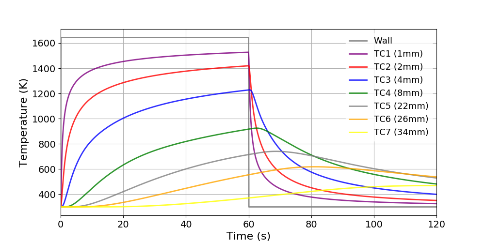
Thermal response of AblationTestCase_1.0 case

AblationTestCase_1.0_equilibriumElementConservation

The AblationTestCase_1.0_equilibriumElementConservation tutorial computes the 1D thermal response of the TACOT material using the elemental mass conservation (Fig. 1.4). Table 1.2 shows the summary of the material sub-models used in this case. Listing [lis:1.0_elem] shows the porousMatProperties file and the different user material sub-models.

Summary of the material sub-models

Model/Tutorial	AblationTestCase_1.0_equiElemCons
Mass
Energy
IO
Gas Properties
Material Properties
Pyrolysis
MaterialChemistry
TimeControl

IO {
  probingFunctions (plotDict surfacePatchDict);
}
Mass {
  MassType DarcyLaw;
}
Energy {
  EnergyType Pyrolysis;
}
GasProperties {
  GasPropertiesType Equilibrium;
}
MaterialChemistry {
  MaterialChemistryType EquilibriumElement;
  mixture tacotair;
}
MaterialProperties {
  MaterialPropertiesType Porous;
  MaterialPropertiesDirectory
  "$PATO_DIR/data/Materials/Composites/TACOT";
}
Pyrolysis {
  PyrolysisType LinearArrhenius;
}
TimeControl {
  TimeControlType GradP;
  chemTransEulerStepLimiter no;
}

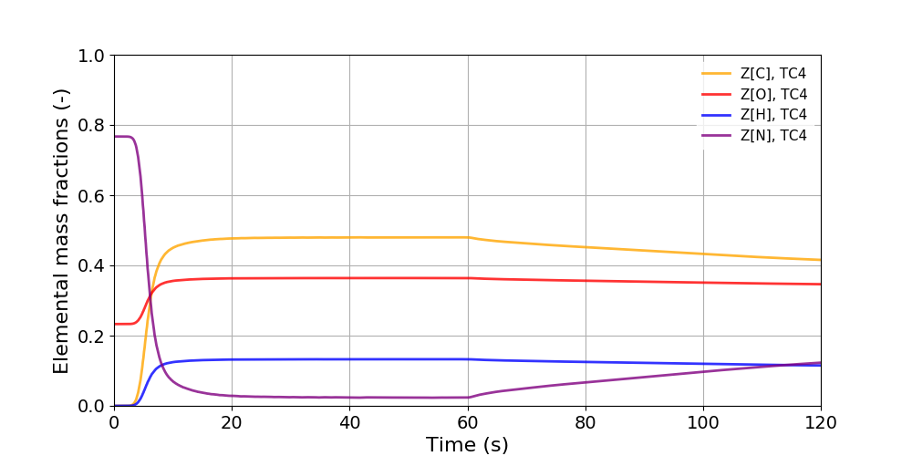
Temporal evolution of the elemental mass fractions

AblationTestCase_1.0_grading

The AblationTestCase_1.0_grading tutorial computes the 1D thermal response of a porous material with a graded phase (Fig. 1.5). Table 1.3 shows the summary of the material sub-models used in this case. Listing [lis:1.0_grading] shows the porousMatProperties file and the different user material sub-models. Listing [lis:1.0_grading_2] and [lis:1.0_grading_3] show the grading properties file and the related gradedTACOT constant properties. The phase 3 has a graded volume fraction from 0.1 to 0.02 for the first in-depth millimeter in the y-axis.

Summary of the material sub-models

Model/Tutorial	AblationTestCase_1.0_grading
Mass
Energy
IO
Gas Properties
Material Properties
Pyrolysis
TimeControl

IO {
  IOType Profile;
  topPatch top;
  bottomPatch bottom;
  plot1DProfileList (eps_s_phase1 eps_s_phase2 eps_s_phase3);
  plot1DMassLoss yes;
  probingFunctions (plotDict surfacePatchDict);
}
Mass {
  MassType DarcyLaw;
}
Energy {
  EnergyType Pyrolysis;
}
GasProperties {
  GasPropertiesType Tabulated;
  GasPropertiesFile
  "$PATO_DIR/data/Materials/Composites/TACOT/gasProperties";
}
MaterialProperties {
  MaterialPropertiesType GradedPorous;
  MaterialPropertiesDirectory
  "$PATO_DIR/data/Materials/Composites/TACOT";
}
Pyrolysis {
  PyrolysisType LinearArrhenius;
}
TimeControl {
  TimeControlType GradP;
  chemTransEulerStepLimiter no;
}

//  d(m)    epsI(-)
    0.05     0.1
    0.049    0.02

// grading prop. file name (distance and volume fraction)
gradingFileEpsI[3] "$FOAM_CASE/constant/grading";
// axis of the grading
gradingAxisEpsI[3] (0 1 0);

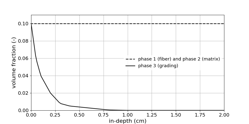
1D profile of the phases’ volume fraction

AblationTestCase_1.0_multiPorousMat

The AblationTestCase_1.0_multiPorousMat tutorial computes the 1D thermal response and the boundary interface between 2 porous materials: TACOT and Cork (Fig. 1.6). Listing [lis:1.0_multiPorous3] shows the mappedWall type in the boundary file of the porousMat1 polyMesh.

porousMat1_to_porousMat2
{
    type            mappedWall;
    inGroups        1(wall);
    nFaces          1;
    startFace       100;
    sampleMode      nearestPatchFace;
    sampleRegion    porousMat2;
    samplePatch     porousMat2_to_porousMat1;
}

Listing [lis:1.0_multiPorous] shows the boundary type of the pressure boundary field (Eq. [eq:bc_coupledMixed]).

\[\tens{\gamma}^S_i = \frac{1}{2} \left( \tens{\gamma}_i + \tens{\gamma}_i^T \right)\]

\[\label{eq:bc_coupledMixed} p_{1/2} = \frac{\frac{\tens{\gamma}^S_2}{\Delta x_2}}{\frac{\tens{\gamma}^S_1}{\Delta x_1} + \frac{\tens{\gamma}^S_2}{\Delta x_2}} ~ p_{1} + \left(1 - \frac{\frac{\tens{\gamma}^S_2}{\Delta x_2}}{\frac{\tens{\gamma}^S_1}{\Delta x_1} + \frac{\tens{\gamma}^S_2}{\Delta x_2}} \right) ~ p_2\]

boundaryField {
    porousMat1_to_porousMat2  {
      type            coupledMixed;
      value           uniform 300;
      Tnbr            p;
      kappaMethod     lookup;
      kappa           Gamma_symm;
    }
}

Thermal response of two adjacent porous materials

AblationTestCase_2.x

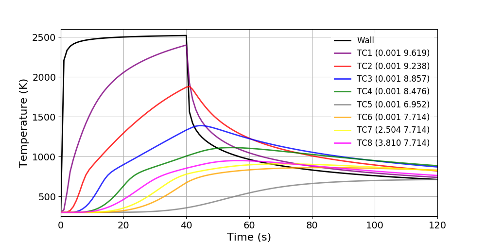
The AblationTestCase_2.x tutorial computes the 1D thermal response of the TACOT material using the surface mass and energy balance boundary conditions (Fig. 1.7). Listing [lis:2.x] shows the boundary type of the temperature boundary field (Eq. [eq:bc_bprime]). Listing [lis:2.x_2] shows a part of the BoundaryConditions file. During the first 0.1 s, the recovery enthalpy (\(h_r\)) varies from 0 to 1.5 MJ \(\cdot\) kg\(^{-1}\) and the heat transfer coefficient (\(C_H\)) from 3 to 300 kg \(\cdot\) m\(^{-2}\) \(\cdot\) s\(^{-1}\). The pressure (\(p = 101325\) Pa), the radiative heat flux (\(q_{rad} =\) 0 W \(\cdot\) m\(^{-2}\)), the blowing correction coefficient (\(\lambda = 0.5\)) and the background temperature (\(T_\infty = 300\) K) stay constant during the simulation. Listing [lis:2.x_3] shows the dynamic mesh flag that allows the boundary to move over time following the boundary conditions type (Eq. [eq:mesh1]).

\[\begin{split}\begin{aligned} \begin{split} \label{eq:bc_bprime} T_{w} = T_{int} + \frac{\Delta x_1}{\boldsymbol{n} \cdot \tens{k_w} \cdot \boldsymbol{n}} (&C'_H \left( h_e - h_w \right) + \dot{m}_{pg} \left( h_{pg} - h_w \right) + \dot{m}_{ca} \left( h_{ca} - h_w \right) \\ & - \varepsilon_w \sigma \left( T_w^4 - T_{\infty}^4 \right) + \alpha_w q_{pla} ) \end{split} \end{aligned}\end{split}\]

\[\label{eq:mesh1} \boldsymbol{v}_{mesh} = \frac{C'_H ~ B'_{ca} }{\rho_{sw} } ~ \vect{n}\]

boundaryField {
    top {
        type Bprime;
        mixtureMutationBprime tacot26;
        environmentDirectory
        "$PATO_DIR/data/Environments/RawData/Earth";
        mappingType constant;
        mappingFileName
        "constant/porousMat/BoundaryConditions";
        mappingFields
        ((rhoeUeCH "1") (h_r "2") (heatOn "3"));
        p 101325;
        qRad 0;
        lambda 0.5;
        Tbackground 300;
        value uniform 300;
    }
}

// t(s)    CH(kg/m2/s)    h_r(J/kg)  heatOn(-)
   0        0.3e-2         0           1
   0.1      0.3            1.5e6       1

movingMesh yes;

Thermal response of AblationTestCase_2.x case

AblationTestCase_2.x_chemistryOff

The AblationTestCase_2.x_chemistryOff tutorial computes the 1D thermal response of the TACOT material using the surface mass and energy balance and energy balance boundary condition without surface chemistry (Fig. 1.8). Listing [lis:2.x_ChemOff] shows the boundary type of the temperature boundary field (Eq. [eq:bc_bprime_ChemOff]).

\[\label{eq:bc_bprime_ChemOff} T_{w} = T_{int} + \frac{\Delta x_1}{\boldsymbol{n} \cdot \tens{k_w} \cdot \boldsymbol{n}} - \varepsilon_w \sigma \left( T_w^4 - T_{\infty}^4 \right) + \alpha_w q_{pla}\]

boundaryField {
    top {
        type Bprime;
        mixtureMutationBprime tacot26;
        environmentDirectory
        "$PATO_DIR/data/Environments/RawData/Earth";
        movingMesh yes;
        mappingType constant;
        mappingFileName
        "constant/porousMat/BoundaryConditions";
        mappingFields
        (
            (p "1")
            (rhoeUeCH "2")
            (h_r "3")
            (hconv "4")
            (Tedge "5")
            (chemistryOn "6")
            );
        qRad 0;
        lambda 0.5;
        Tbackground 300;
        value uniform 300;
    }
}

Thermal response of AblationTestCase_2.x_chemistryOff case

AblationTestCase_2.x_equilibriumElementConservation

The AblationTestCase_2.x_equilibriumElementConservation tutorial computes the 1D thermal response of the TACOT material using the boundary type and the material sub-models from Table 1.2.

AblationTestCase_2.x_inDepthOxidation

The AblationTestCase_2.x_inDepthOxidation tutorial computes the 1D thermal response of the TACOT material, including in-depth oxidation (Fig. 1.9). Table 1.4 shows the summary of the material sub-models used in this case. Listing [lis:2.x_oxi] shows the porousMatProperties file and the different user material sub-models.

Summary of the material sub-models

Model/Tutorial	AblationTestCase_2.x_inDepthOxidation
IO
Material Properties
Pyrolysis
Mass
Energy
Gas Properties
Material Chemistry
Volume Ablation
TimeControl

IO {
  IOType Profile;
  topPatch "top";
  bottomPatch "bottom";
  plot1DProfileList (Y[O2]);
  plot1DMassLoss yes;
  probingFunctions (plotDict surfacePatchDict);
}
MaterialProperties {
  MaterialPropertiesType Porous;
  MaterialPropertiesDirectory
  "$PATO_DIR/data/Materials/Composites/TACOT_newChemistry";
  detailedSolidEnthalpies yes;
}
Pyrolysis {
  PyrolysisType LinearArrhenius;
}
Mass {
  MassType DarcyLaw_Heterogeneous;
}
Energy {
  EnergyType Pyrolysis_Heterogeneous_SpeciesDiffusion;
}
GasProperties {
  GasPropertiesType FiniteRate;
}
MaterialChemistry {
  MaterialChemistryType SpeciesConservation;
  mixture TACOT_oxidation_species;
}
VolumeAblation {
  VolumeAblationType FibrousMaterialTypeA;
}
TimeControl {
  TimeControlType GradP_ChemYEqn;
  chemTransEulerStepLimiter no;
}

Thermal response including in-depth oxidation

AblationTestCase_2.x_multiMat

The AblationTestCase_2.x_multiMat tutorial computes the 1D thermal response of 1 porous and 2 non-porous materials. Listing [lis:2.x_multiMat1] shows the regionProperties file that selects the 3 different materials: porousMat, subMat1 and subMat2. Table 1.5 shows the summary of the subMat1 material sub-models used in this case. Listing [lis:2.x_multiMat] shows the subMat1Properties file and the different user material sub-models.

regions (solid (porousMat subMat1 subMat2));

Summary of the subMat1 material sub-models

Model/Tutorial	AblationTestCase_2.x_multiMat
Energy
Material Properties

Energy {
  EnergyType PureConduction;
}
MaterialProperties {
  MaterialPropertiesType Fourier;
  MaterialPropertiesDirectory
  "$PATO_DIR/data/Materials/Fourier/FourierTemplate";
}

CarbonFiberOxidation

The CarbonFiberOxidation tutorial computes the 1D in-depth oxidation of the CarbonFiberPreform material (Fig. 1.10 and 1.11). Table 1.6 shows the summary of the material sub-models used in this case. Listing [lis:carOxi] shows the porousMatProperties file and the different user material sub-models.

Summary of the material sub-models

Model/Tutorial	AblationTestCase_2.x_inDepthOxidation
IO
Material Properties
Pyrolysis
Mass
Gas Properties
Material Chemistry
Volume Ablation
TimeControl

IO {
  IOType Profile;
  topPatch "top";
  bottomPatch "bottom";
  plot1DProfileList (Y[O2] Y[CO2] rho_s);
  plot1DMassLoss yes;
  probingFunctions (plotDict surfacePatchDict);
}
MaterialProperties {
  MaterialPropertiesType Porous;
  MaterialPropertiesDirectory
  "$PATO_DIR/data/Materials/Composites/CarbonFiberPreform";
  detailedSolidEnthalpies yes;
}
Pyrolysis {
  PyrolysisType LinearArrhenius;
}
Mass {
  MassType DarcyLaw_Heterogeneous;
}
GasProperties {
  GasPropertiesType FiniteRate;
}
MaterialChemistry {
  MaterialChemistryType SpeciesConservation;
  mixture Carbon_oxidation_species;
}
VolumeAblation {
  VolumeAblationType FibrousMaterialTypeA;
  energyConservation isothermal;
}
TimeControl {
  TimeControlType GradP_ChemYEqn;
  chemTransEulerStepLimiter no;
}

Temporal and in-depth profile of the solid density

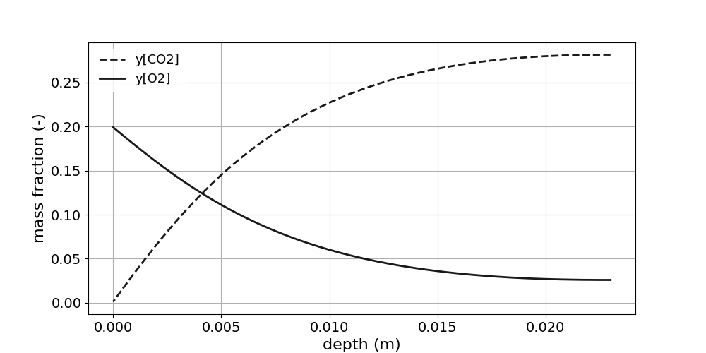
In-depth profile of the gaseous mass fractions

Listing [lis:carOxi2] shows the CHEMKIN input file for the material chemistry model. There are 3 elements, 5 species and 1 finite-rate reaction (Eq. [eq:fr1]).

\[\label{eq:fr1} k_1(T) = 5\cdot10^7 ~ T^0 ~ \text{exp}\left(\frac{T}{28600}\right)\]

ELEMENTS
 C  N  O
END
SPECIES
 N2  O2  CO2  CO  C(gr)
END
REACTIONS
  C(gr) + O2 => CO2     5e7   0   28680
END

PorousStorage_1D

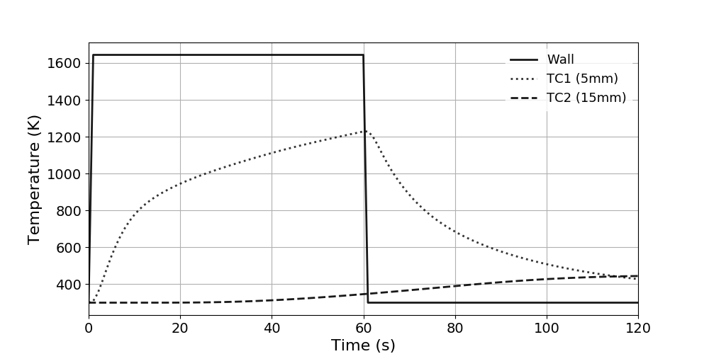
The PorousStorage_1D tutorial computes the 1D thermal response of a quartzite bed. The singleGraph file produces the 1D plot (Fig. 1.12). The Ta and Tg files respectively the initialization of the solid temperature field and the gazeous temperature field. Table 1.7 show the summary of the material sub-models used in this case. Listing [lis:porousStorage] shows the porousMatProperties file ans the different user material sub-models.

Summary of the material sub-models

Model/Tutorial	PorousStorage_1D
Mass
Energy
IO
Gas Properties
Material Properties
Pyrolysis
TimeControl

IO {
  writeFields (U vG);
  probingFunctions (plotDict);
}
Pyrolysis {
  PyrolysisType virgin;
}
Mass {
  MassType DarcyLaw2T;
}
Energy {
  EnergyType Pyrolysis2T;
}
GasProperties {
  GasPropertiesType Tabulated2T;
  GasPropertiesFile
  "$PATO_DIR/data/Materials/Granular/Quartzite_bed/gasProperties_with_k";
}
MaterialProperties {
  MaterialPropertiesType Porous;
  MaterialPropertiesDirectory
  "$PATO_DIR/data/Materials/Granular/Quartzite_bed";
}
TimeControl {
  TimeControlType GradP;
  chemTransEulerStepLimiter no;
}

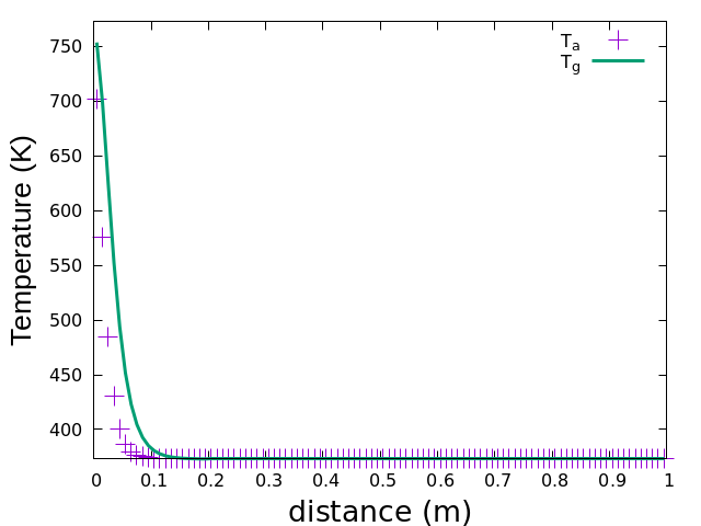
Solid and gaz temperatures at \(t = 60\) s

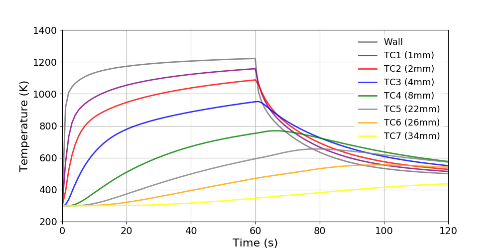
PureConduction

The PureConduction tutorial computes the 1D thermal response of the TACOT material using the pure conduction model. Table 1.8 shows the summary of the material sub-models used in this case. Listing [lis:pureCond] shows the porousMatProperties file and the different user material sub-models.

Summary of the material sub-models

Model/Tutorial	AblationTestCase_2.x_inDepthOxidation
IO
Energy
Material Properties
Pyrolysis

IO {
  probingFunctions (plotDict surfacePatchDict);
}
Energy {
  EnergyType PureConduction;
}
MaterialProperties {
  MaterialPropertiesType PureConduction;
  MaterialPropertiesDirectory
  "$PATO_DIR/data/Materials/Composites/TACOT";
}
Pyrolysis {
  PyrolysisType virgin;
}

StartdustAtmosphericEntry

The StartdustAtmosphericEntry tutorial computes the 1D thermal response of the TACOT material using the surface mass and energy balance boundary conditions during the Stardust atmospheric entry (Fig. 1.13).

Thermal response of the Stardust atmospheric entry

WoodPyrolysis

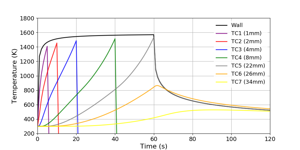
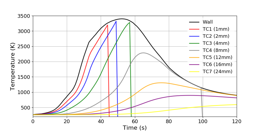
The WoodPyrolysis tutorial computes the 1D thermal response of the Wood material (Fig. 1.14). Table 1.9 shows the summary of the material sub-models used in this case. Listing [lis:wood] shows the porousMatProperties file and the different user material sub-models.

Summary of the material sub-models

Model/Tutorial	WoodPyrolysis
IO
Pyrolysis
Mass
Energy
Gas Properties
Material Properties
TimeControl

IO {
  probingFunctions (plotDict surfacePatchDict);
}
Pyrolysis {
  PyrolysisType LinearArrhenius;
}
Mass {
  MassType DarcyLaw;
}
Energy {
  EnergyType Pyrolysis;
}
GasProperties {
  GasPropertiesType Tabulated;
  GasPropertiesFile
  "$PATO_DIR/data/Materials/Wood/Generic/gasProperties";
}
MaterialProperties {
  MaterialPropertiesType Porous;
  MaterialPropertiesDirectory
  "$PATO_DIR/data/Materials/Wood/Generic"
  detailedSolidEnthalpies yes;
}
TimeControl {
  TimeControlType GradP;
}

Temporal evolution of the temperature in the Wood

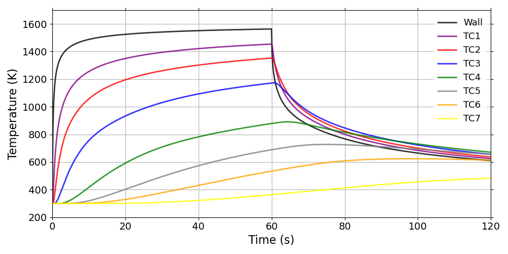
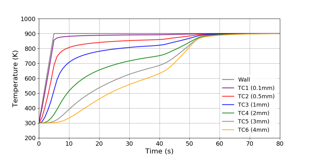
WoodPyrolysisCylinder1D

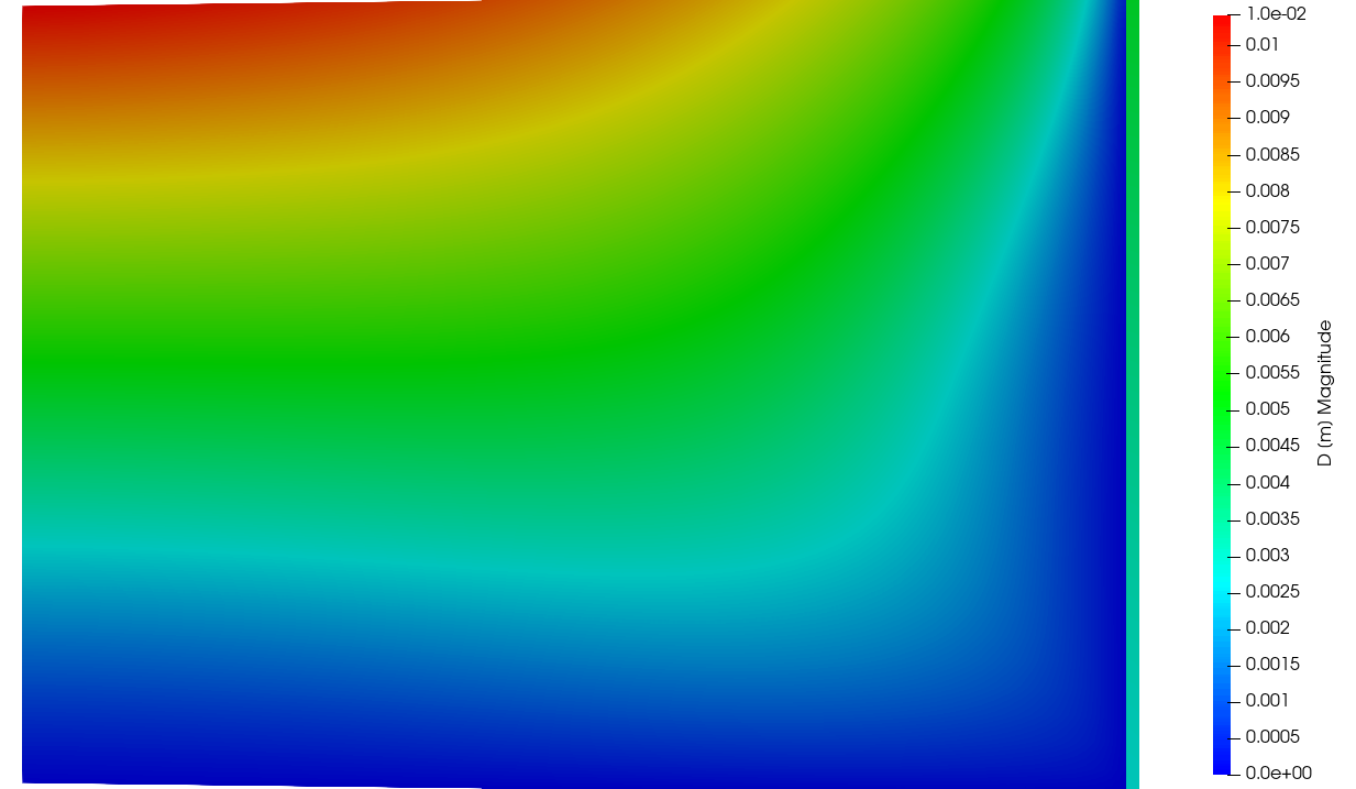
The WoodPyrolysisCylinder1D computes the 1D-axisymetric thermo-mechanical response of the Wood material (Fig. 1.15). Table 1.10 shows the summary of the material sub-models used in this case. Listing [lis:woodCylinder] shows the porousMatProperties file and the different user material sub-models.

Summary of the material sub-models

Model/Tutorial	WoodPyrolysisCylinder1D
IO
Pyrolysis
Mass
Energy
Gas Properties
Material Properties
TimeControl

IO {
  probingFunctions (plotDict surfacePatchDict);
   writeFields (tau D E alpha sigma epsilon);
}
Pyrolysis {
  PyrolysisType LinearArrhenius;
}
Mass {
  MassType DarcyLaw;
}
Energy {
  EnergyType Pyrolysis;
}
SolidMechanics
{
    SolidMechanicsType  Displacement;
    planeStress         true;
}
GasProperties {
  GasPropertiesType Tabulated;
  GasPropertiesFile
  "$PATO_DIR/data/Materials/Wood/GenericUNC/gasProperties";
}
MaterialProperties {
  MaterialPropertiesType Porous;
  MaterialPropertiesDirectory
  "$PATO_DIR/data/Materials/Wood/GenericUNC"
  detailedSolidEnthalpies yes;
}
TimeControl {
  TimeControlType GradP;
}

Temporal evolution of the temperature in the Wood

2D tutorials

Figure 1.16 shows the architecture of the 2D tutorials. The inputs and expected outputs of the 2D tutorials are described below.

AblationTestCase_3.x

The AblationTestCase_3.x tutorial computes the 2D thermal response of the TACOT material (Fig. 1.17 and 1.18). Listing [lis:3.x] shows the pressure boundary field of 2D-axi_pressureMap type. Listing [lis:3.x_2] and [lis:3.x_3] show examples of the fluxFactorMap and BoundaryConditions files. The pressure boundary field values follow the Equation [eq:pxt] during the first 0.1 s at a distance up to 70 \(\mu\)m from fluxFactorCenter in the fluxFactorNormal direction.

\[\label{eq:pxt} p(x,t) = \left(\frac{10132.5 - 405.3}{0.1}~ t + 405.3 \right) \left[ 1 - \frac{1 - 0.998}{0.00007} ~ x \right]\]

\[\text{\hspace{0.2cm} t = [}0,0.1\text{],~~ x = [}0,7\cdot10^{-5}]\]

boundaryField{
    top {
        type boundaryMapping;
        mappingType "2D-axi_pressureMap";
        mappingFileName
        "constant/porousMat/BoundaryConditions";
        mappingFields ((p  "1"));
        fluxFactorNormal (0 -1 0);
        fluxFactorCenter (0.0 0.1 0.0);
        fluxFactorProjection no;
        fluxFactorMapFileName
        "constant/porousMat/fluxFactorMap";
        dynamicPressureFieldName p_dyn;
        pointMotionDirection (0 -1 0);
        fluxFactorThreshold
        fluxFactorThreshold [ 0 0 0 0 0 0 0 ] 0.97;
        value uniform 405.3;
    }
}

// t(s)   p_total_w(Pa)
    0       405.3
    0.1     10132.5

//  d(m)        fluxFactor      pressureFactor
    0               1               1
    0.00007         1               0.998

Thermal response of the AblationTestCase_3.x

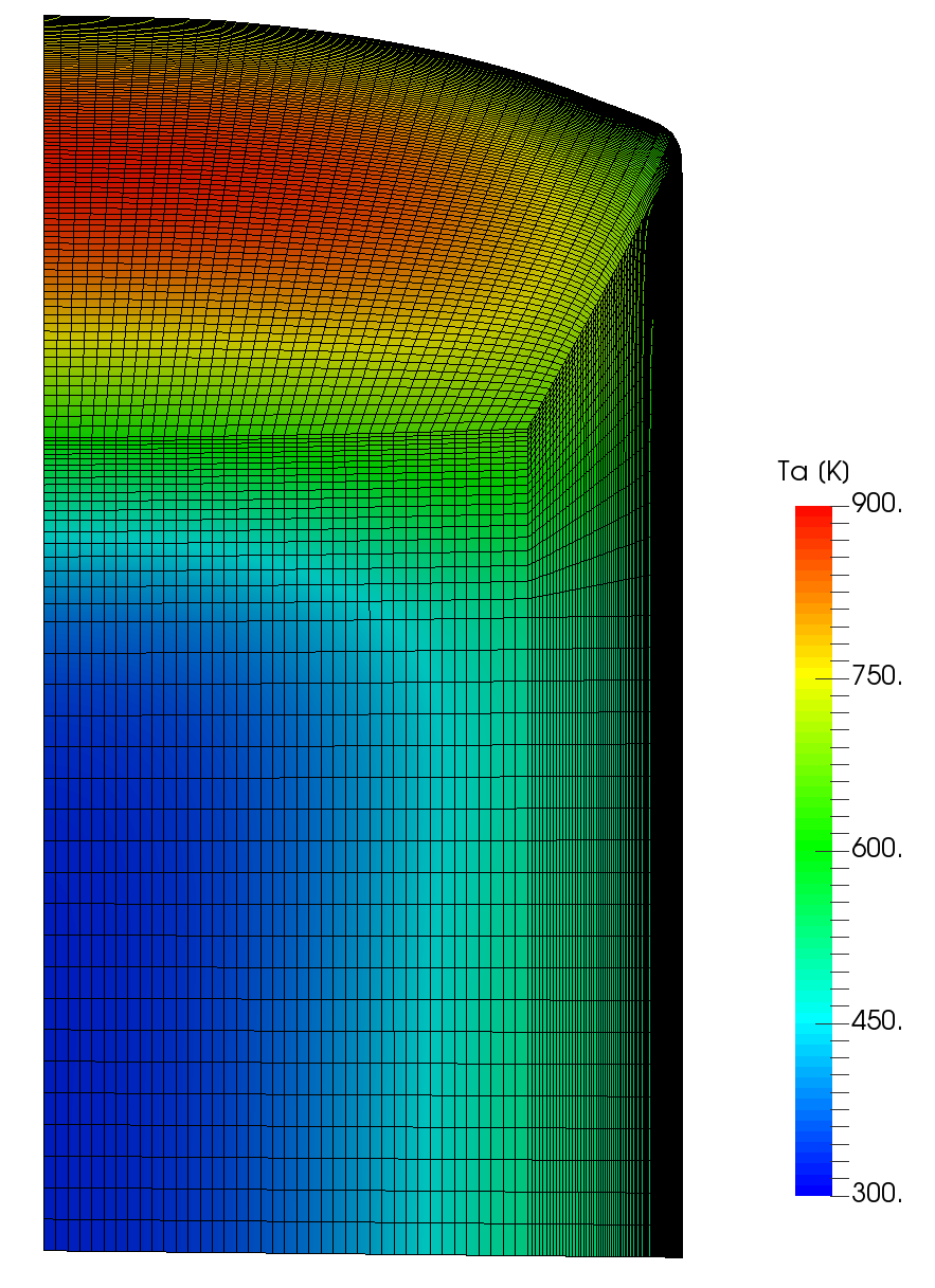
2D Ta profile of the AblationTestCase_3.x (120 s)

AblationTestCase_3.x_multiMat

The AblationTestCase_3.x_multiMat tutorial computes the 2D thermal response of 1 porous and 1 non-porous materials. Listing [lis:3.x_multiMat1] shows the regionProperties file that selects the 2 different materials: porousMat and subMat1 (Fig. 1.19). Table 1.11 shows the summary of the subMat1 material sub-models used in this case. Listing [lis:3.x_multiMat] shows the subMat1Properties file and the different user material sub-models. Listing [lis:3.x_multiMat_2] shows the temperature boundary field of “radiative” type (subsection [subsec:BC:radiative]). The radiative heat flux (\(q_{rad} = 0\) W \(\cdot\) m\(^{-2}\)) and the background temperature (\(T_\infty = 300\) K) are constant during the simulation. The heat transfer coefficient and the recovery enthalpy varies linearly over time following the BoundaryConditions file.

regions (solid (porousMat subMat1));

Summary of the subMat1 material sub-models

Model/Tutorial	AblationTestCase_3.x_multiMat
Energy
Material Properties

Energy {
  EnergyType PureConduction;
}
MaterialProperties {
  MaterialPropertiesType Fourier;
  MaterialPropertiesDirectory
  "$PATO_DIR/data/Materials/Fourier/FourierTemplate";
}

boundaryField {
    top {
        type radiative;
        mappingType constant;
        mappingFileName
        "constant/subMat1/BoundaryConditions";
        mappingFields ((rhoeUeCH "1") (h_r "2")
        );
        qRad 0;
        Tbackground 300;
        value uniform 300;
    }
}

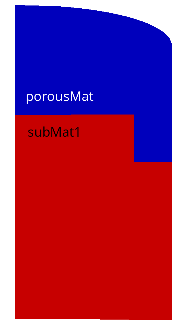
Regions of the AblationTestCase_3.x_multiMat

ArcJet_cylinder

The ArcJet_cylinder tutorial computes the 2D thermal response of the TACOT material (Fig. 1.20). This case uses the same inputs than .

2D Ta profile of the Arcjet_cylinder (120 s)

DemiseTestCase_1.0

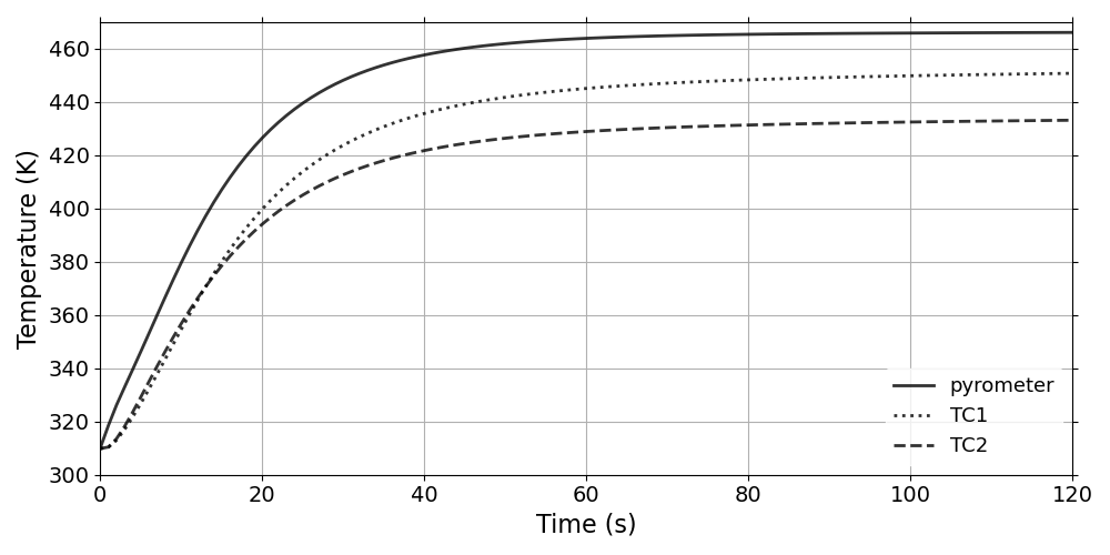
The DemiseTestCase_1.0 tutorial computes the 2D axisysmetric thermal response of AISI 316L stainless steel mounted on a cork material (Fig. 1.21 and 1.22). Listing [lis:Demise1.0] shows the temperature coupling boundary condition inside the demiseMat. Table 1.12 shows the summary of the demiseMat material sub-models used in this case. Table 1.13 presents the summary of the porousMat material submodels.

boundaryField{
  demiseMat_to_porousMat
  {
    type            compressible::turbulentTemperatureCoupledBaffleMixed;
    value           uniform 310;
    Tnbr        Ta;
    kappaMethod     lookup;
    kappa           k_abl_sym;
  }
}

Summary of the demiseMat sub-models

Model/Tutorial	DemiseTestCase_1.0: demiseMat
IO
Energy
Material Properties

Summary of the porousMat sub-models

Model/Tutorial	DemiseTestCase_1.0: porousMat
IO
Pyrolysis
Mass
Energy
Gas Properties
Material Properties
TimeControl

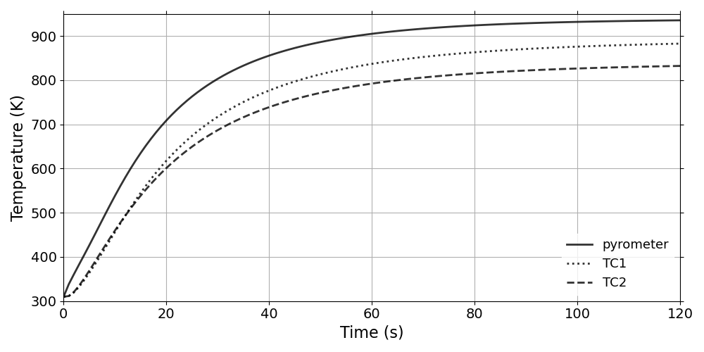
Thermal response of the DemiseTestCase_1.0

2D Ta profile of the DemiseTestCase_1.0 (276 s)

DemiseTestCase_1.0_coupled_constantFluidThermo

The DemiseTestCase_1.0_coupled_constantFluidThermo tutorial computes the 2D axisymetric thermal response of AISI 316L stainless steel protected by a silicon carbide cap and a porous cork holder inside the hot gas flow (Fig. 1.23 and 1.24). Listing [lis:Demise1.0coupled] shows the temperature coupling boundary condition between the demise material and the hot gas flow. Listing [lis:demiseSetCase] presents the setCase file. Tables 1.14, 1.15, and 1.16 shows the summary of the ceramicMat, demiseMat, and porousMat respectively.

boundaryField{
  demiseMat_to_hotFlow
  {
    type            compressible::turbulentTemperatureRadCoupledMixed;
    Tnbr            T;
    kappaMethod     lookup;
    kappa       k_abl_sym;
    QrNbr           none;
    Qr              Qr;
    value           uniform 310;
  }
}

fluidType chtMultiRegionFoam;

Summary of the ceramicMat sub-models

Model/Tutorial	DemiseTestCase_1.0_coupled_constantFluidThermo: ceramicMat
IO
Energy
Material Properties

Summary of the demiseMat sub-models

Model/Tutorial	DemiseTestCase_1.0_coupled_constantFluidThermo: demiseMat
IO
Energy

Summary of the porousMat sub-models

Model/Tutorial	DemiseTestCase_1.0_coupled_constantFluidThermo: porousMat
IO
Pyrolysis
Mass
Energy
Gas Properties
Material Properties
TimeControl

Thermal response of the DemiseTestCase_1.0_coupled_constantFluidThermo

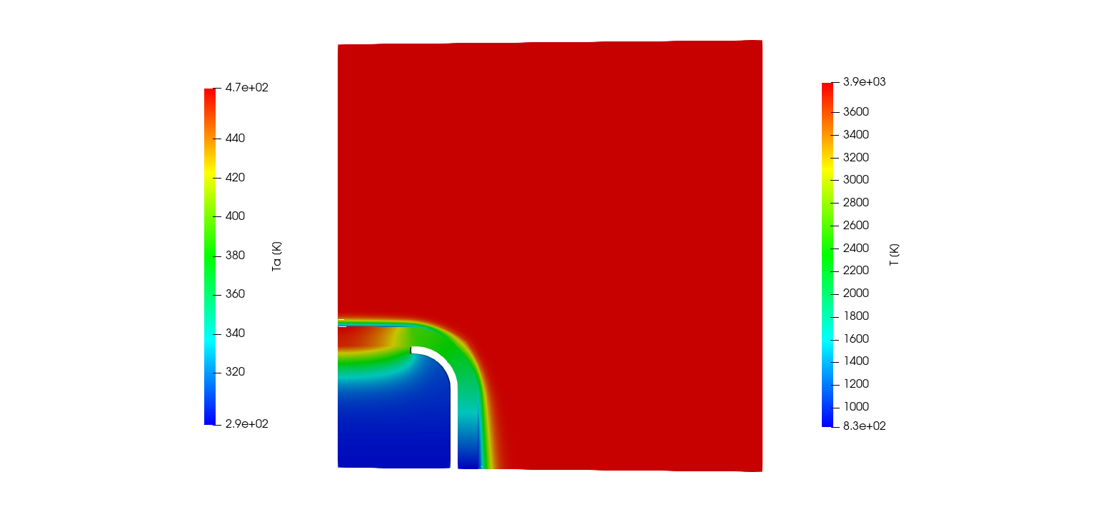
2D Ta profile of the DemiseTestCase_1.0_coupled_constantFluidThermo (120 s)

DemiseTestCase_1.0_coupled_equilibriumFluidChemistry

The DemiseTestCase_1.0_coupled_equilibriumFluidChemistry tutorial computes the 2D axisymetric thermal response of AISI 316L stainless steel protected by a silicon carbide cap and a porous cork holder inside the hot gas flow in chemical equilibrium (Fig. 1.25 and 1.28). Listing [lis:demiseEquil] shows the thermophysicalProperties file for the hotFlow.

thermoType {
  type            heRhoThermo;
  mixture         pureMixture;
  transport       tabular;
  thermo          hTabular;
  equationOfState Rhotabular;
  specie          specie;
  energy          sensibleEnthalpy;
}

mixture {
  specie
  {
    nMoles          1;
    molWeight       28.96;
  }

  equationOfState
  {
    file "$PATO_DIR/data/Fluids/fluidPropertyTable/Air5/Equilibrium/densityTable";
    outOfBounds clamp;
  }

  thermodynamics
  {
    Hf 0;
    Cp
    {
      file "$PATO_DIR/data/Fluids/fluidPropertyTable/Air5/Equilibrium/cpTable";
      outOfBounds clamp;
    }
    h
    {
      file "$PATO_DIR/data/Fluids/fluidPropertyTable/Air5/Equilibrium/hTable";
      outOfBounds clamp;
    }
  }

  transport
  {
    mu
    {
      file "$PATO_DIR/data/Fluids/fluidPropertyTable/Air5/Equilibrium/muTable";
      outOfBounds clamp;
    }

    kappa
    {
      file "$PATO_DIR/data/Fluids/fluidPropertyTable/Air5/Equilibrium/kappaTable";
      outOfBounds clamp;
    }
  }
}

Thermal response of the DemiseTestCase_1.0_coupled_equilibriumFluidChemistry

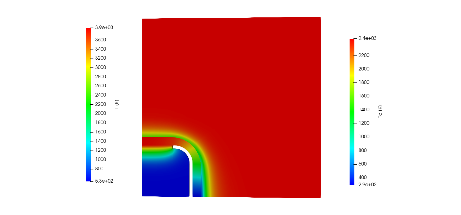
2D Ta profile of the DemiseTestCase_1.0_coupled_equilibriumFluidChemistry (120 s)

DemiseTestCase_1.0_coupled_frozenFluidChemistry

The DemiseTestCase_1.0_coupled_frozenFluidChemistry tutorial computes the 2D axisymetric thermal response of AISI 316L stainless steel protected by a silicon carbide cap and a porous cork holder inside the chemically frozen hot gas flow (Fig. 1.27 and 1.28).

Thermal response of the DemiseTestCase_1.0_coupled_frozenFluidChemistry

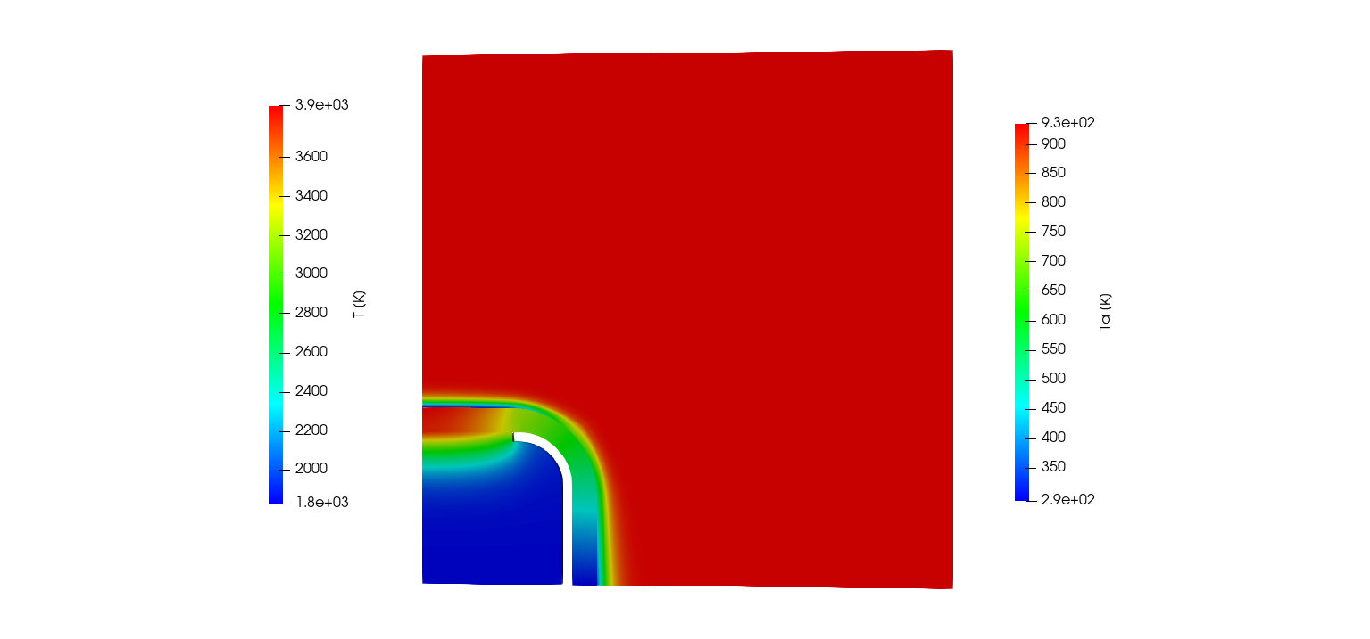
2D Ta profile of the DemiseTestCase_1.0_coupled_frozenFluidChemistry (120 s)

FlappingConsole

The FlappingConsole tutorial computes the fluid solid interaction response of a solid console immersed into a flow (Fig. 1.29). Listing [lis:flapping] shows the fluid_to_solid cellMotionU boundary condition, and listing [lis:flapping_2] presents the solid_to_fluid D boundary condition.

boundaryField{
    fluid_to_solid
    {
        type            codedFixedValue;
        value           uniform (0 0 0);
        name            solidfollowing;
        code
        #{
            vectorField n(this->patch().nf());
            scalar deltaT = this->db().time().deltaTValue();
            const mappedPatchBase& mpp =
                refCast<const mappedPatchBase>(this->patch().patch());
            const polyMesh& nbrMesh = mpp.sampleMesh();

            const label samplePatchI = mpp.samplePolyPatch().index();
            const fvPatch& nbrPatch =
                refCast<const fvMesh>(nbrMesh).boundary()[samplePatchI];

            const fvPatchField<vector>& nbrField =
                nbrPatch.lookupPatchField
                <
                    GeometricField<vector, fvPatchField, volMesh>,
                    vector
                >
                ("deltaD");

            tmp<Field<vector>> nbrIntFld
            (
                new Field<vector>(nbrField.size(), pTraits<vector>::zero)
            );
            nbrIntFld.ref() = nbrField.patchInternalField();
            vectorField deltaD = nbrIntFld.ref();
            operator==(deltaD/deltaT);
        #};

        codeInclude
        #{
            #include "mappedPatchBase.H"
        #};

        codeOptions
        #{
            -I$(LIB_SRC)/meshTools/lnInclude
        #};
    }
}

boundaryField{
    fluid_to_solid
    {
        type            codedFixedValue;
        value           uniform (0 0 0);
        name            solidfollowing;
        code
        #{
            vectorField n(this->patch().nf());
            scalar deltaT = this->db().time().deltaTValue();
            const mappedPatchBase& mpp =
                refCast<const mappedPatchBase>(this->patch().patch());
            const polyMesh& nbrMesh = mpp.sampleMesh();

            const label samplePatchI = mpp.samplePolyPatch().index();
            const fvPatch& nbrPatch =
                refCast<const fvMesh>(nbrMesh).boundary()[samplePatchI];

            const fvPatchField<vector>& nbrField =
                nbrPatch.lookupPatchField
                <
                    GeometricField<vector, fvPatchField, volMesh>,
                    vector
                >
                ("deltaD");

            tmp<Field<vector>> nbrIntFld
            (
                new Field<vector>(nbrField.size(), pTraits<vector>::zero)
            );
            nbrIntFld.ref() = nbrField.patchInternalField();
            vectorField deltaD = nbrIntFld.ref();
            operator==(deltaD/deltaT);
        #};

        codeInclude
        #{
            #include "mappedPatchBase.H"
        #};

        codeOptions
        #{
            -I$(LIB_SRC)/meshTools/lnInclude
        #};
    }
}

Velocity of the fluid and displacement of the solid for the FlappingConsole case.

FlowTube2T

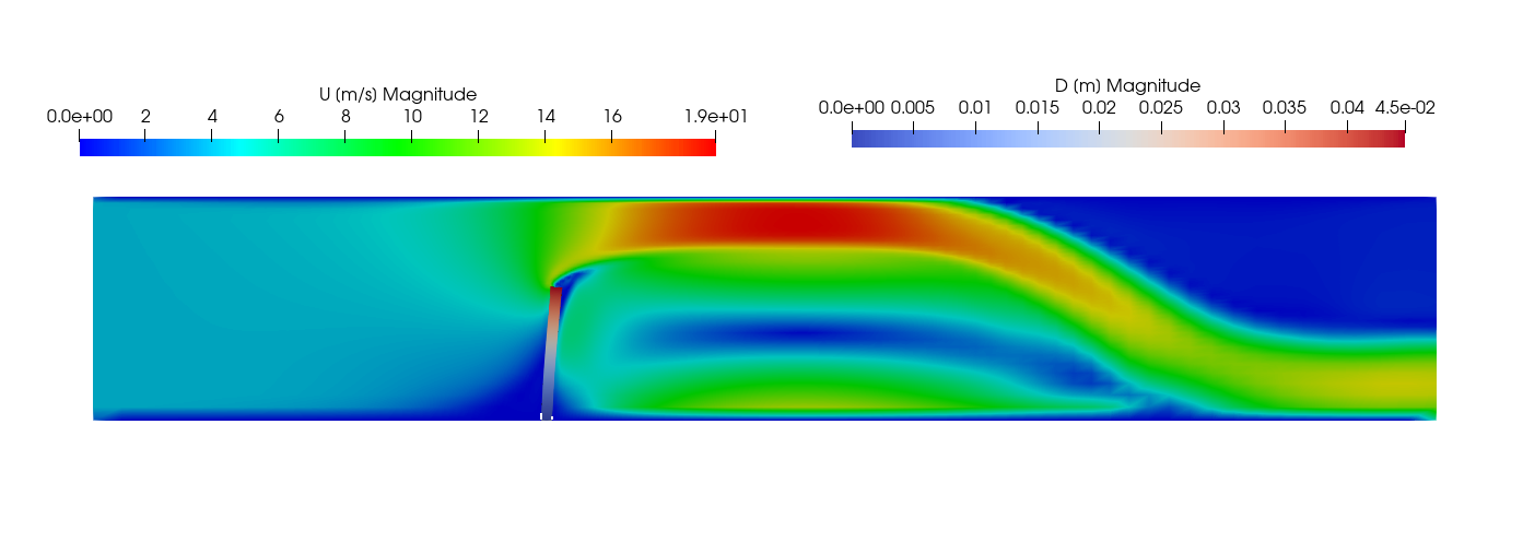
the FlowTube2T tutorial computes the 2D thermal response of a porous medium heated by a gas flow (Fig. 1.30). Table 1.17 shows the summary of the porousMat material used in this case.

Summary of the porousMat sub-models

Model/Tutorial	FlowTube2D: porousMat
IO
Pyrolysis
Mass
Energy
Gas Properties
Material Properties
TimeControl

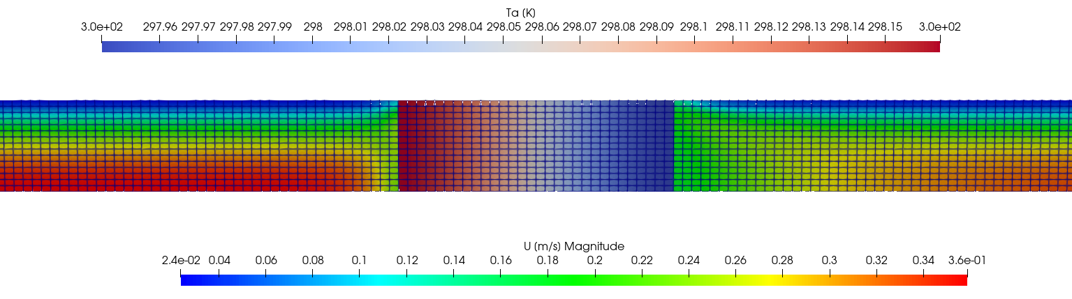
Velocity of the fluid and thermal response of the porous material for the FlowTube2T case.

ImmersedCylinder_Full_chtMultiRegionFoam

The ImmersedCylinder_Full_chtMultiRegionFoam tutorial computes the 2D thermal response of TACOT material inside a hot gas flow (Fig 1.31 and 1.32). Listing [lis:immersedFullcht] shows the pressure coupling boundary condition between the porous material and the hot gas flow.

boundaryField{
porousMat_to_flow
  {
    type        fixedValueToNbrValue;
    nbr         p;
    value       $internalField;
  }
}

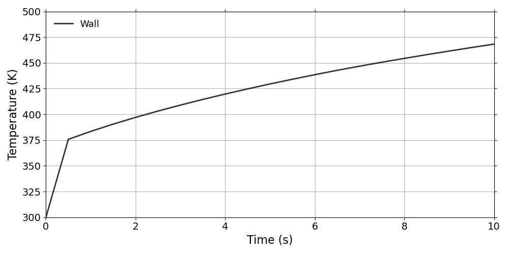
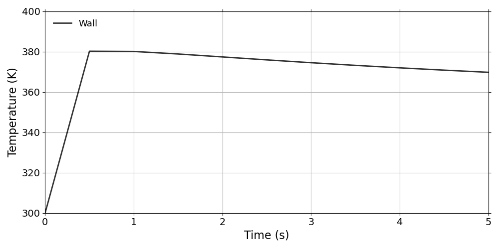
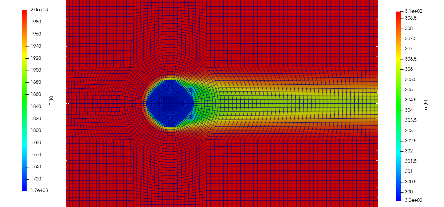
Thermal response of the ImmersedCylinder_Full_chtMultiRegionFoam

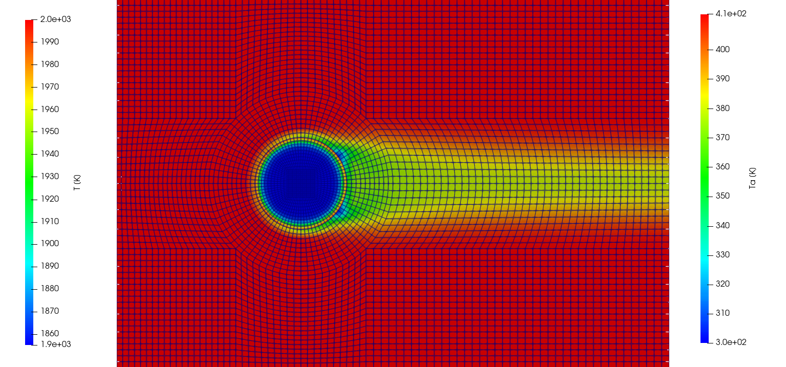
2D temperature profile of the ImmersedCylinder_Full_chtMultiRegionFoam (10 s)

ImmersedCylinder_Full_reactingFoam

The ImmersedCylinder_Full_reactingFoam tutorial computes the 2D thermal response of TACOT material inside a reactive hot gas flow (Fig. 1.33 and 1.34). Listing [lis:immersedFullreact] shows the thermophyscialProperties file for the flow.

thermoType {
  type            heRhoThermo;
  mixture         reactingMixture;
  transport       sutherland;
  thermo          janaf;
  energy          sensibleEnthalpy;
  equationOfState perfectGas;
  specie          specie;
}

inertSpecie CO2;

chemistryReader foamChemistryReader;

foamChemistryFile "$FOAM_CASE/constant/flow/reactions";

foamChemistryThermoFile "$FOAM_CASE/constant/flow/thermo.compressibleGas";

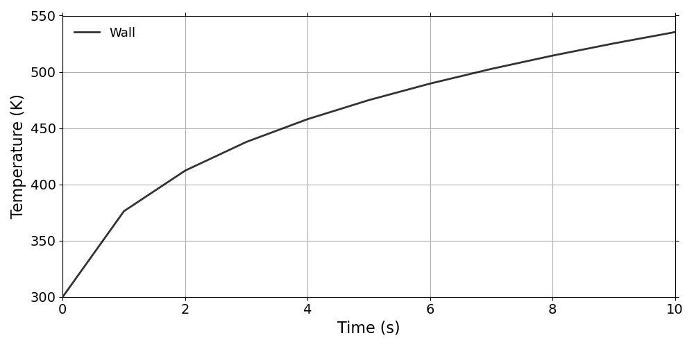
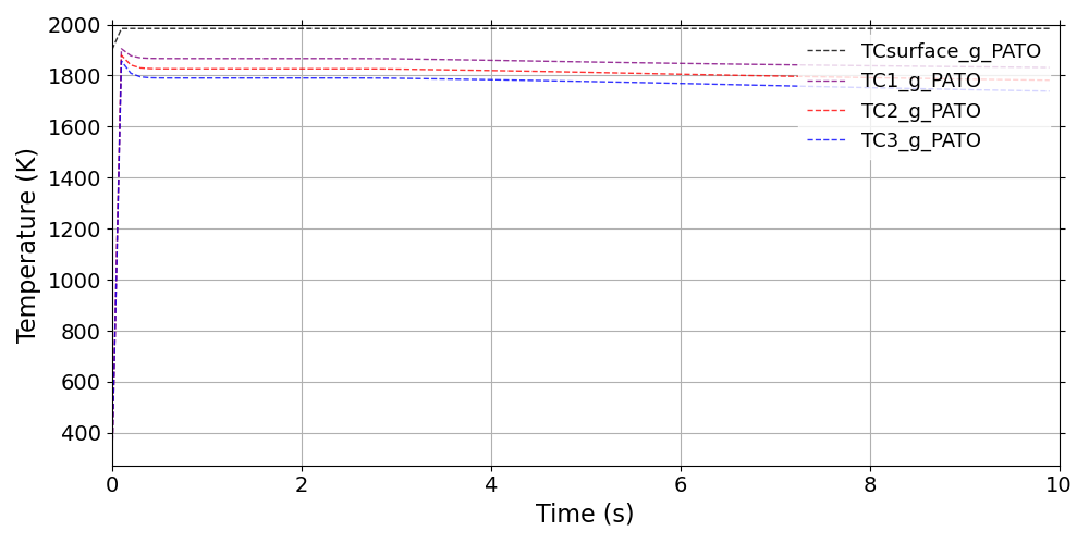
Thermal response of the ImmersedCylinder_Full_reactingFoam

2D temperature profile of the ImmersedCylinder_Full_reactingFoam (5 s)

ImmersedCylinder_Quarter_chtMultiRegionFoam

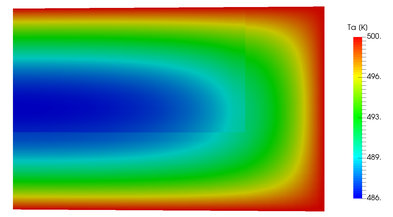
The ImmersedCylinder_Quarter_chtMultiRegionFoam tutorial computes the 2D symmetric thermal response of TACOT material inside a hot gas flow (Fig 1.35 and 1.36).

Thermal response of the ImmersedCylinder_Quarter_chtMultiRegionFoam

2D temperature profile of the ImmersedCylinder_Quarter_chtMultiRegionFoam (10 s)

Ma5ArcJetOnPorousFlatPlate

The Ma5ArcjetOnPorousFlatPlate computes the 2D thermal response of a plate of TACOT material inside a supersonic (\(Ma = 5\)) arc jet (Figure 1.37 and 1.38). It is possible to run simulations on each zone (fluid or porousMaterial) separately for uncoupled simulations or on both mesh simultaneously for coupled simulations. 4 Allrun files are available:

• Allrun_aero: run the Mach-5 flow simulation alone on a single processor with rhoCentralFoam solver from OpenFOAM under frozen chemistry assumption.

• Allrun_parallel_aero: run the Mach-5 flow simulation in parallel with rhoCentralFoam solver from OpenFOAM. The simulation takes 8 hours on 192 processors to reach the final time of 0.004 s.

• Allrun_coupled_standard: run the coupled simulation using a 2 temperatures model for the porous material. The flow is initialized with a converged solution.

• Allrun_coupled_stitching: run the coupled simulation with a time scale splitting strategy to speed-up convergence. This method use the experimental solver PATOxs.

Gas thermal response of the Ma5ArcJetOnPorousFlatPlate

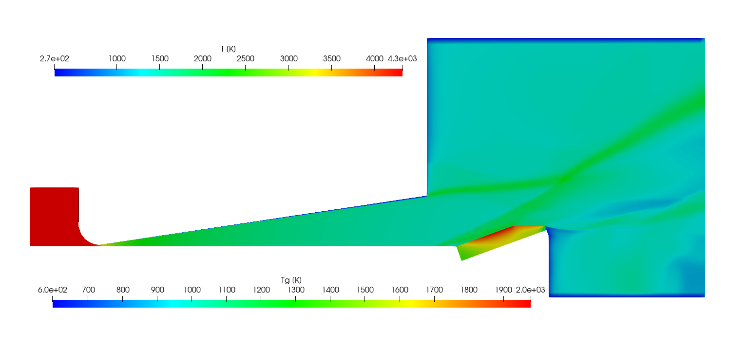
2D gas temperature profile of the Ma5ArcJetOnPorousFlatPlate

OpenCylinder

The OpenCylinder tutorial compute the 2D thermo-mechanical response of a solid cylinder (Fig 1.39 and 1.40). A computation of the analytical solution is included in the tutorial (Eq. [eq:analyticalT] to Eq. [eq:analyticalSigma]).

\[\label{eq:analyticalT} T = \frac{\left( T_{in} - T_{out}\right)}{ln\left( \frac{0.7}{0.5} \right) } ~ ln \left( \frac{0.7}{r} \right)\]

\[\sigma_R = \frac{\alpha ~ E ~ (Ti_{in} - T_{out})}{2(1 - \nu) ~ ln \left( \frac{0.7}{0.5} \right)} ~ \left( -ln \left( \frac{0.7}{r} \right) - \frac{0.5^2}{0.7^2 -0.5^2} ~ \left( 1 - \frac{0.7}{r} \right) ln \left( \frac{0.7}{0.5} \right) \right)\]

\[\sigma_{\Theta} = \frac{\alpha ~ E ~ (Ti_{in} - T_{out})}{2(1 - \nu) ~ ln \left( \frac{0.7}{0.5} \right)} ~ \left( 1 - ln \left( \frac{0.7}{r} \right) - \frac{0.5^2}{0.7^2 -0.5^2} ~ \left( 1 + \frac{0.7}{r} \right) ln \left( \frac{0.7}{0.5} \right) \right)\]

\[\label{eq:analyticalSigma} \sigma_z = 0.3 ~ \left( \sigma_R + \sigma_{\Theta} \right) - E ~ \alpha ~ T\]

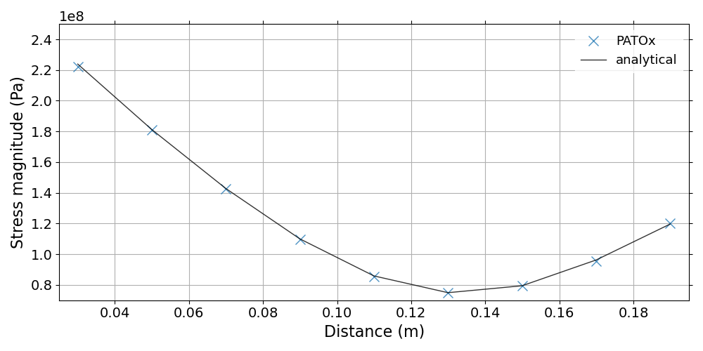
Stress response of the OpenCylinder

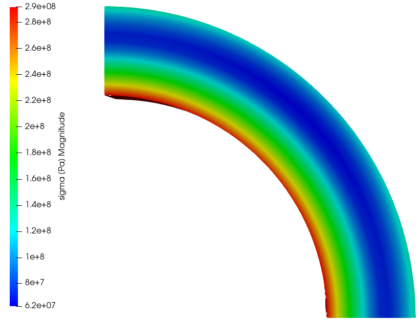
2D stress magnitude profile of the OpenCylinder

Poiseuille_flow

The Poiseuille_flow tutorial computes the 2D axisymetric, incompressible, laminar Poiseuille flow and compares it with analytical results (Fig 1.41).

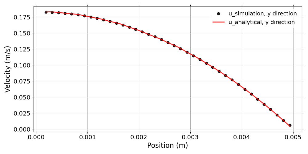
Velocity of the flow for the Poiseuille_flow tutorial

QuartziteBed_thermal_load

The QuartziteBed_thermal_load tutorial computes the 2D axisymetric thermo-mechanical response of the Quartzite bed material enclosed in a 16Mo3 steel (Fig 1.42). The 2 temperature thermal load is precalculated in the thermalLoad directory. Table 1.18 shows the summary of the porousMat material used in this case and Table 1.19 presents the summary of the tank material used in this case. Mechanical contact between the two material is not taken into account. There are only separated by difference in thermo-mechanical properties

Summary of the porousMat sub-models

Model/Tutorial	QuartziteBed_thermal_load: porousMat
IO
Pyrolysis
Material Properties
SolidMechanics

Summary of the tank sub-models

Model/Tutorial	QuartziteBed_thermal_load: tank
IO
Pyrolysis
Material Properties
SolidMechanics

2D displacement profile of the QuartziteBed_thermal_load

TGA_standardCrucible

The TGA_standardCrucible tutorial computes the 2D thermal response of the TACOT material (Fig. 1.43). This case uses the same inputs as .

2D Ta profile of the TGA_standardCrucible (10 s)

WoodPyrolysis_cylinder

The WoodPyrolysis_cylinder tutorial computes the 2D thermal response of the TACOT material (Fig. 1.44). This case uses the same inputs as .

2D Ta profile of the WoodPyrolysis_cylinder (30 s)

3D tutorials

Figure 1.45 shows the architecture of the 3D tutorials. The inputs and expected outputs of the 3D tutorials are described below.

ArcJet_cylinder_3D

The Arcjet_cylinder_3D tutorial computes the 3D thermal response of the TACOT material (Fig. 1.46). This case uses the same inputs as .

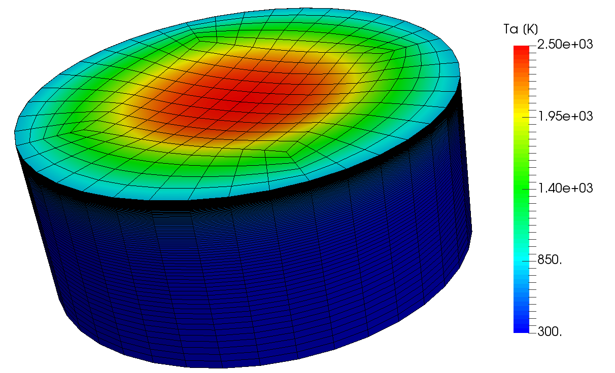
3D material response of the Arcjet_cylinder (120 s)

MSL_monolithic

The MSL_monolithic tutorial computes the 3D thermal response of the monolithic heat shield of the Mars Science Laboratory (MSL) made of TACOT material during Mars atmosphere entry (Fig. 1.47). Listing [lis:MSL] shows the temperature boundary field of BC type using the 3D-tecplot type. The pressure, the heat transfer coefficient and the recovery enthalpy are linearly interpolated from the DPLR-MSL_* Tecplot files.

boundaryField {
    top {
        type Bprime;
        BprimeFile
        "$FOAM_CASE/data/Materials/TACOT-Mars/BprimeTable";
        mappingType "3D-tecplot";
        mappingFileName
        "$FOAM_CASE/data/Environment/DPLR-MSL";
        mappingSymmetry y;
        mappingFields ((p "1") (rhoeUeCH "2") (h_r "3"));
        Tbackground 187;
        qRad 0;
        lambda 0.5;
        heatOn 1;
        value uniform 300;
    }
}

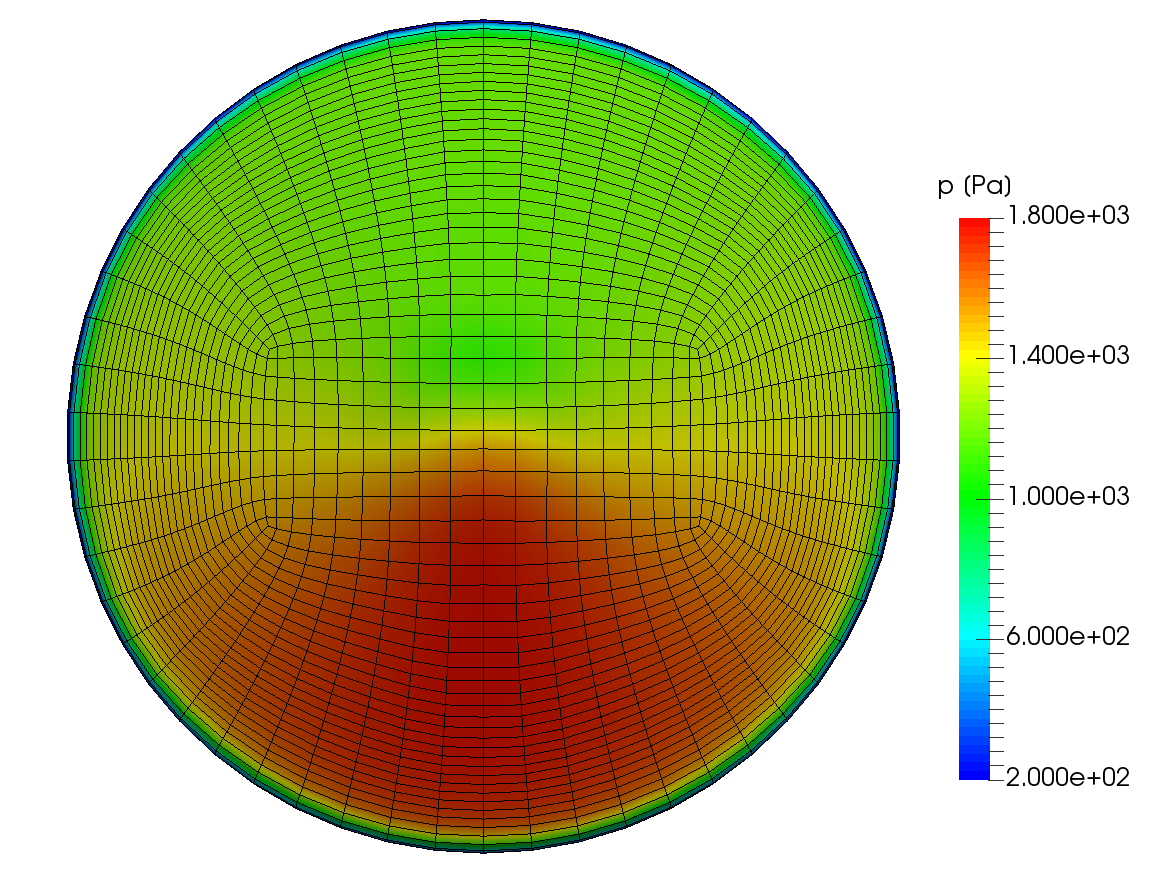
3D material response of the MSL_monolithic (100 s)

Flow_Around_Sphere

The flow_Around_Sphere tutorial computes the 3D incompressible, laminar flow around a sphere and computes drag and lift coefficients (Fig 1.48).

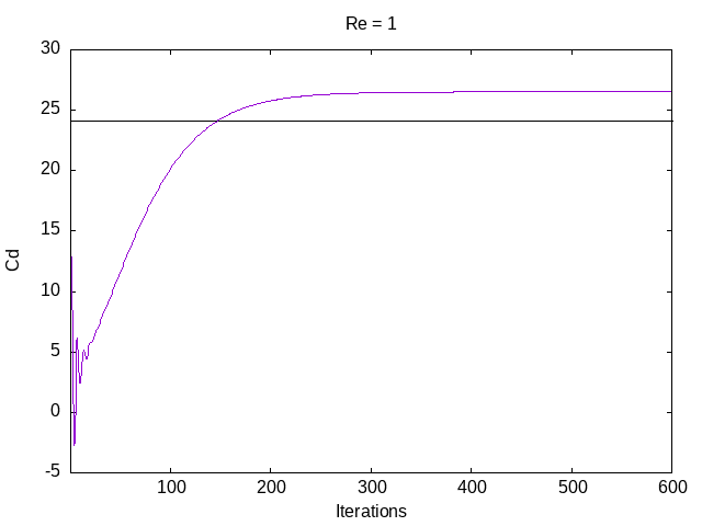
Drag coefficient of a sphere from Flow_Around_Sphere