Material Model
The creation of models, fields, and properties are described in the PATOx output during the initialization of the MaterialModel. An example is given in Fig. 1.1.
Example: initialization of the porousMat MaterialModel.
Mass Model
no Type
The no type is empty and serves as a place holder when the is not used.
DarcyLaw Type
The DarcyLaw type solves the semi-implicit pressure equation (Eq. [eq:p1]). This equation comes from the perfect gas law (Eq. [eq:perfectGasLaw]), the mass conservation (Eq. [eq:m1]) and the Darcy’s law (Eq. [eq:darcy]). The right-hand side is the total pyrolysis gas production term and is computed in the . The gaseous thermodynamic and transport properties are computed in the . The solid material properties are computed in the .
}{mu_g ~ R ~ T_a} ~ boldsymbol{partial_x} ~ p_g right) = pi_{tot}
DarcyLaw_Heterogeneous Type
The DarcyLaw_Heterogeneous type solves the semi-implicit pressure equation (Eq. [eq:p2]), based on the DarcyLaw type. The heterogeneous production rate (Eq. [eq:omegaH]), updated in the , is added as source term in the right-hand side.
}{mu_g ~ R ~ T_a} ~ boldsymbol{partial_x} ~ p_g right) = pi_{tot} + Omega_h
DarcyLaw2T Type
The DarcyLaw2T type solves the semi-implicit pressure equation (Eq. [eq:p3]), based on the DarcyLaw type. Porous material is considered in thermal non-equilibrium (\(T_g \ne T_s \ne T_a\)) and gaseous temperature is used instead of porous material equilibrium temperature.
}{mu_g ~ R ~ T_g} ~ boldsymbol{partial_x} ~ p_g right) = pi_{tot}
DarcyForchheimerLaw Type
The DarcyForchheimerLaw type solves the semi-implicit pressure equation (Eq. [eq:p4]). This equation comes from the perfect gas law (Eq. [eq:perfectGasLaw]), the mass conservation (Eq. [eq:m1]) and the Darcy-Forchheimer’s law (Eq. [eq:forchheimer]). The tensor :math:`\underline{\underline{X_s}} ` (Eq. `[eq:permeabilityInv] <#eq:permeabilityInv>`__) is introduced for convenience.
}{R ~ T_a} ~ ~ boldsymbol{partial_x} ~ p_g right) = pi_{tot}
DarcyForchheimerLaw2T Type
The DarcyForchheimerLaw2T type solves the semi-implicit pressure equation (Eq. [eq:p5]), based on the DarcyForchheimerLaw type. Porous material is considered in thermal non-equilibrium (\(T_g \ne T_s \ne T_a\)) and gaseous temperature is used instead of porous material equilibrium temperature.
}{R ~ T_g} ~ ~ boldsymbol{partial_x} ~ p_g right) = pi_{tot}
FixedPressureGamma Type
The FixedPressureGamma type fixes the value of the pressure field, the gamma (Eq. [eq:gamma]) field and the boundary conditions. The user can modify the following inputs in the model properties file:
internalField_P = internal cell center value of the scalar pressure.
boundaryField_P = boundary face center value of the scalar pressure.
internalField_Gamma = internal cell center value of the tensor gamma.
boundaryField_Gamma = boundary face center value of the tensor gamma.
Energy Model
no Type
The no type is empty and serves as a place holder when the is not used.
PureConduction Type
The PureConduction type updates the temperature by solving the energy equation (Eq. [eq:PureCond]). The solid material properties are computed in the .
Pyrolysis Type
The Pyrolysis type updates the temperature by solving the energy equation (Eq. [eq:EnergyPyro]). The left-hand side is composed by the solid and gaseous storage, the solid thermal conduction, the gaseous thermal convection and the pyrolysis energy flux. The gaseous thermodynamic and transport properties are computed in the . The solid material properties and the pyrolysis energy flux are computed in the .
Pyrolysis_Heterogeneous_SpeciesDiffusion Type
The Pyrolysis_Heterogeneous_SpeciesDiffusion type updates the temperature by solving the energy equation (Eq. [eq:EnergyPyroHetero]) based on the type. The heterogeneous energy flux (Eq. [eq:heteroEnergy]) and the energy flux transported by diffusion of the gaseous species (Eq. [eq:DiffEnergy]) are added as source term to the right-hand side.
Pyrolysis2T Type
The Pyrolysis2T type updates the solid temperature and the gas temperature by solving two energy equation (Eq. [eq:EnergyPyro2T]). The left-hand side of Eq. [eq:EnergyPyro2Ts] is composed by the solid storage, the solid thermal conduction, the pyrolysis energy flux and the exchange between solid and fluid. The left-hand side of Eq. [eq:EnergyPyro2Tg] is composed by the gaseous storage, the pressure energy, the gaseous convection, the gas thermal conduction and the exchange between solid and fluid. The gaseous thermodynamic and transport properties are computed in the . The solid material properties and the pyrolysis energy flux are computed in the .
ForchheimerPyrolysis Type
The ForchheimerPyrolysis type updates the temperature by solving the energy equation (Eq. [eq:EnergyForchPyro]) based on the type with gaseous thermal convection term calculated by Eq. [eq:gammaHgForch].
}{R ~ T_a}
ForchheimerPyrolysis2T Type
The ForchheimerPyrolysis2T type updates the solid temperature and the gas temperature by solving two energy equation (Eq. [eq:EnergyForchPyro2T]) based on the type with gaseous thermal convection term calculated by Eq. [eq:gammaHgForch2T].
}{R ~ T_g}
Darcy2T Type
The Darcy2T type updates the temperature by solving energy equations (Eq. [eq:EnergyDarcy2T]) based on the type with constant solid heat capacity for materials without pyrolysis.
Forchheimer2T Type
The Forchheimer2T type is identical to the type and will be deleted in a future release.
CorrectBC Type
The CorrectBC type updates all the boundary conditions of the temperature.
BoundaryTable Type
The BoundaryTable type updates the internal cell center value of the temperature using the value of the uniformFixedValue boundary face.
FixedTemperature Type
The FixedTemperature type fixes the value of the temperature fields and boundary conditions. The user can modify the following inputs in the model properties file:
internalField_T = internal cell center value of the temperature.
boundaryField_T = boundary face center value of the temperature.
TabulatedTemperature Type
The TabulatedTemperature type fixes the value of the temperature fields from an external file and boundary conditions from the inputs. Internal fields are mapped from a tabulated value and a distance from a given patch. The user can modify the following inputs in the model properties file:
internalFieldTable_fileName = file containing table of internal cell center value of the temperature.
originPatchName = name of the patch from which the temperature values will be mapped.
boundaryField_T = boundary face center value of the temperature.
ControlTemperature Type
The ControlTemperature type fixes a linear time dependent value of temperature inside the domain (Eq. [eq:controlTemperature]). The user can modify the following inputs in the model properties file:
a = temperature at \(t = 0\).
b = slope factor.
Input/Output (IO) Model
no Type
The no type writes the fields from the writeFields input following the controlDict file and writes the probing fields from the probingFunctions input to the output folder.
PurePyrolysis Type
The PurePyrolysis type computes the solid density ratio of virgin and char (Eq. [eq:rhoRatio]) and the normalized total pyrolysis production rate (Eq. [eq:NormPi]) in function of time. This type compares also \(r(t)\) and \(\widetilde{\pi}_{tot}(t)\) to reference files and gives the least square difference (Eq. [eq:LSD]).
InverseProblem Type
The InverseProblem type takes a user list of fields and reference files to compare. Then, this type computes the least square difference (Eq. [eq:LSD2]).
Profile Type
The Profile type takes a user list of fields. Then, this types computes and writes the 1D in-depth profile of these fields.
LinearInterpolation Type
The LinearInterpolation type initializes the fields from a user list with a linear interpolation (Eq. [linInt]).
mass Type
The Mass type computes the gas mass flow rate at the surface, the char mass flow rate, the total recession of the material and the position when the sample reached \(2\)% and \(98\)% of the charred state.
WriteControl Type
The WriteControl type writes the fields from IO:writeFields at the additional times provided in additionalWriteTimes. This type also writes the probing fields from IO:probingFunctions at the additional times provided in additionalProbingTimes. The user can modify the following inputs in the model properties file:
additionalWriteTimes = list of additional times to write the fields.
additionalProbingTimes = list of additional times to write the probing fields.
Volume Ablation Model
no Type
The no type is empty and serves as a place holder when the is not used.
FibrousMaterialTypeA Type
The FibrousMaterialTypeA type updates the solid volume fraction by solving the Equation [eq:eps_s]. This equation includes the external solid density (Eq. [eq:rho_ext]) and the heterogeneous production rate (Eq. [eq:omegaH2]), updated in the model. The fiber radius (Eq. [eq:rT]), the specific surface (Eq. [eq:ss]), the site density (Eq. [eq:sd]) and the solid carbon mass fraction (Eq. [eq:yc]) are then computed in function of the solid volume fraction.
Gas Properties Model
no Type
The no type is empty and serves as a place holder when the is not used.
Equilibrium Type
The Equilibrium type updates the following gaseous transport and thermodynamic properties in function of pressure, temperature and elemental mole composition using the library. The total advancement of pyrolysis (\(\tau\)) is computed in the . The virgin and charred properties are given by the user in the constant material properties file, read in the .
The gaseous molar mass, \(M_g\)
The gaseous enthalpy, \(h_g\)
The gaseous viscosity, \(\mu_g\)
The gaseous density, \(\rho_g\)
The gaseous volume fraction, \(\epsilon_g = \epsilon_{g,c} + (\epsilon_{g,v} - \epsilon_{g,c})~ \tau\)
FiniteRate Type
The FiniteRate type updates the following gaseous transport and thermodynamic properties in function of pressure, temperature and species mass composition using the library. The total advancement of pyrolysis (\(\tau\)) is computed in the . The virgin and charred properties are given by the user in the constant material properties file, read in the .
The gaseous molar mass, \(M_g\)
The gaseous enthalpy, \(h_g\)
The gaseous viscosity, \(\mu_g\)
The gaseous density, \(\rho_g\)
The gaseous volume fraction, \(\epsilon_g = \epsilon_{g,c} + (\epsilon_{g,v} - \epsilon_{g,c})~ \tau\)
Energy flux transported by diffusion of the species, \(\dot{E}_{D}\)
Tabulated Type
The Tabulated type updates the following gaseous transport and thermodynamic properties in function of pressure and temperature using a linear interpolation method and a table given by the user. The total advancement of pyrolysis (\(\tau\)) is computed in the . The virgin and charred properties are given by the user in the constant material properties file, read in the .
The gaseous molar mass, \(M_g\)
The gaseous enthalpy, \(h_g\)
The gaseous viscosity, \(\mu_g\)
The gaseous density, \(\rho_g\)
The gaseous volume fraction, \(\epsilon_g = \epsilon_{gc,} + (\epsilon_{g,v} - \epsilon_{g,c})~ \tau\)
Tabulated2T Type
The Tabulated2T type updates the following gaseous transport and thermodynamic properties in function of pressure and gas temperature using a linear interpolation method and a table given by the user. The total advancement of pyrolysis (\(\tau\)) is computed in the . The virgin and charred properties are given by the user in the constant material properties file, read in the .
The gaseous molar mass, \(M_g\)
The gaseous enthalpy, \(h_g\)
The gaseous viscosity, \(\mu_g\)
The gaseous thermal conductivity \(k_g\)
The gaseous density, \(\rho_g\)
The gaseous volume fraction, \(\epsilon_g = \epsilon_{gc,} + (\epsilon_{g,v} - \epsilon_{g,c})~ \tau\)
Material Properties Model
no Type
The no type is empty and serves as a place holder when the is not used.
Fourier Type
The Fourier type updates the following solid properties (if they already exist in the mesh) using the Fourier’s law.
The solid thermal conductivity, :math:`underline{underline{K_s}}
= sum^{N_c}_{i=0} ~ k_i ~ T^i`
The solid heat capacity, \(c_{p,s} = \sum^{N_c}_{i=0} ~ c_{ps,i} ~ T^i\)
The solid density, \(\rho_s = \sum^{N_c}_{i=0} ~ \rho_{s,i} ~ T^i\)
The solid Young’s modulus \(E_s = \sum^{N_c}_{i=0} ~ E_{s,i} ~ T^i\)
The solid Poisson’s ration \(\nu_s = \sum^{N_c}_{i=0} ~ \nu_{s,i} ~ T^i\)
The solid thermal expansion coefficient \(\alpha_{th} = \sum^{N_c}_{i=0} ~ \alpha_{th,i} ~ T^i\)
The solid Jomaa function \(\xi_s = \sum^{N_c}_{i=0} ~ \xi_{s,i} ~ T^i\)
Fourier_Radiation Type
The Fourier_Radiation type updates the following solid properties (if they already exist in the mesh) using the Fourier’s law.
The solid thermal conductivity, :math:`underline{underline{K_s}}
= sum^{N_c}_{i=0} ~ k_i ~ T^i`
The solid heat capacity, \(c_{p,s} = \sum^{N_c}_{i=0} ~ c_{ps,i} ~ T^i\)
The solid density, \(\rho_s = \sum^{N_c}_{i=0} ~ \rho_{s,i} ~ T^i\)
The solid emissivity, \(\varepsilon_s = \sum^{N_c}_{i=0} ~ \varepsilon_{s,i} ~ T^i\)
The radiative heat flux, \(q_r = - \varepsilon_s \sigma_{SB} \left( T^4 - T_\infty^4 \right)\)
The solid Young’s modulus \(E_s = \sum^{N_c}_{i=0} ~ E_{s,i} ~ T^i\)
The solid Poisson’s ration \(\nu_s = \sum^{N_c}_{i=0} ~ \nu_{s,i} ~ T^i\)
The solid thermal expansion coefficient \(\alpha_{th} = \sum^{N_c}_{i=0} ~ \alpha_{th,i} ~ T^i\)
The solid Jomaa function \(\xi_s = \sum^{N_c}_{i=0} ~ \xi_{s,i} ~ T^i\)
Porous_const Type
The Porous_const type updates the solid properties (if they already exist in the mesh) using constant values from the constantProperties file located in the MaterialPropertiesDirectory folder.
The solid thermal conductivity, \(k_{s,xx} = k_{s,yy} = k_{s,zz} =\) k_const
The solid heat capacity, \(c_{p,s} =\) cp_const
The solid density, \(\rho_s =\) rho_s_const
The solid permeability, \(K_{s,xx} = K_{s,yy} = K_{s,zz} =\) K_const
The solid Forchheimer coefficient, \(\beta_{s,xx} = \beta_{s,yy} = \beta_{s,zz} =\) Beta_const
The pyrolysis energy flux, \(\dot{E}_p =\) pyrolysisFlux_const
The solid emissivity, \(\varepsilon_s =\) emissivity_const
The solid absorptivity, \(\alpha_s =\) absorptivity_const
The solid Young’s modulus \(E_s =\) E_const
The solid Poisson’s ration \(\nu_s =\) nu_const
The solid thermal expansion coefficient \(\alpha_{th} =\) alpha_const
The solid charred enthalpy, \(h_c =\) h_c_const
The solid Jomaa function, \(\xi_s =\) xi_const
Porous Type
The Porous type updates the following solid properties (if they already exist in the mesh) using the solid density and the total advancement of pyrolysis, updated in the .
The solid thermal conductivity, :math:`underline{underline{K_s}}
= tens{k_{sv}} ~ tau ~ frac{rho_{sv}}{maxleft(rho_{s},rho_{sc} right)} + tens{k_{sc}} left(1 - tau ~ frac{rho_{sv}}{maxleft(rho_{s},rho_{sc} right)} right)`
The solid heat capacity, \(c_{p,s} = c_{p,sv}~ \tau~ \frac{\rho_{sv}}{max\left(\rho_{s},\rho_{sc} \right)} + c_{p,sc} \left(1 - \tau ~ \frac{\rho_{sv}}{max\left(\rho_{s},\rho_{sc} \right)} \right)\)
The solid density, \(\rho_s = \sum^{N_p}_i \rho_{s,i} ~ \epsilon_{s,i}\)
The solid phase density, \(\rho_{s,i} = \frac{\epsilon_{sv,i}}{\epsilon_{s,i}} \rho_{sv,i} \left( 1 - \sum^{N_{sp}}_j \cst{F}_{ij} \chi_{ij} \right)\)
The solid permeability, :math:`underline{underline{K_s}}
= tens{K_{sc}} + (tens{K_{sv}} - tens{K_{sc}})~ tau`
The solid Forchheimer coefficient, \(\tens{\beta_s} = \tens{\beta_{sc}} + (\tens{\beta_{sv}} - \tens{\beta_{sc}})~ \tau\)
The solid average enthalpy, \(\bar{h} = \frac{\rho_{sv} h_{sv} -\rho_{sc} h_{sc}}{ \rho_{sv} - \rho_{sc}}\)
The pyrolysis energy flux, \(\dot{E}_p = - \bar{h} \pi_{tot}\)
The solid emissivity, \(\varepsilon_s = \varepsilon_{sv} ~\tau ~ \frac{\rho_{sv}}{max\left(\rho_{s},\rho_{sc} \right)} + \varepsilon_{sc} \left(1 - \tau ~ \frac{\rho_{sv}}{max\left(\rho_{s},\rho_{sc} \right)} \right)\)
The solid absorptivity, \(\alpha_s = \alpha_{sv} ~ \tau ~ \frac{\rho_{sv}}{max\left(\rho_{s},\rho_{sc} \right)} + \alpha_{sc} \left(1 - \tau ~ \frac{\rho_{sv}}{max\left(\rho_{s},\rho_{sc} \right)} \right)\)
The solid Young’s modulus \(E_s = E_{sv} ~\tau + E_{sc} \left( 1 - \tau \right)\)
The solid Poisson’s ration \(\nu_s = \nu_{sv} ~\tau + \nu_{sc} \left( 1 - \tau \right)\)
The solid thermal expansion coefficient \(\alpha_{th} = \alpha_{th,v} ~\tau + \alpha_{th,c} \left( 1 - \tau \right)\)
The solid charred enthalpy, \(h_c\)
The solid Jomaa function, \(\xi_s\)
\[h_{S,s} = \frac{\rho_{sv} \left[ h_{S,sv}(p,T) - h_{Sv}(p,T_0)\right] - \rho_{sc} \left[ h_{S,sc}(p,T) - h_{S,sc}(p,T_0)\right]}{\rho_{sv} - \rho_{sc} }\]\[h_{S,sv} = \int^T_{T_0} c_{p,sv} ~ dT \text{\hspace{2cm}} h_{S,sc} = \int^T_{T_0} c_{p,sc} ~ dT\]\[\dot{E}_p = - \sum^{N_p}_i \sum_j^{N_{sp}} \rho_{sv,i} ~ \epsilon_{sv,i} ~ \cst{F}_{ij} ~ \partial_t \chi_{ij} \left(h_{p,ij} + h_{S,s} \right)\]
GradedPorous Type
The GradedPorous type updates the following solid properties (if they already exist in the mesh) based on the Porous type. The total advancement of pyrolysis (\(\tau\)) is updated in the . Porosity \(\phi\) is calculated from values from a given file at distance from a given patch.
The solid thermal conductivity, :math:`underline{underline{K_s}}
= tens{k_{sv}} ~ tau ~ frac{rho_{sv}}{maxleft(rho_{s},rho_{sc} right)} + tens{k_{sc}} left(1 - tau ~ frac{rho_{sv}}{maxleft(rho_{s},rho_{sc} right)} right)`
The solid heat capacity, \(c_{p,s} = c_{p,sv}~ \tau~ \frac{\rho_{sv}}{max\left(\rho_{s},\rho_{sc} \right)} + c_{p,sc} \left(1 - \tau ~ \frac{\rho_{sv}}{max\left(\rho_{s},\rho_{sc} \right)} \right)\)
The solid density, \(\rho_s = \sum^{N_p}_i \rho_{s,i} ~ \epsilon_{s,i}\)
The solid phase density, \(\rho_{s,i} = \frac{\epsilon_{sv,i}}{\epsilon_{s,i}} \rho_{sv,i} \left( 1 - \sum^{N_{sp}}_j \cst{F}_{ij} \chi_{ij} \right)\)
The solid permeability, :math:`underline{underline{K_s}}
= tens{K_{sc}} + (tens{K_{sv}} - tens{K_{sc}})~ tau`
The solid Forchheimer coefficient, \(\tens{\beta_s} = \tens{\beta_{sc}} + (\tens{\beta_{sv}} - \tens{\beta_{sc}})~ \tau\)
The solid average enthalpy, \(\bar{h} = \frac{\rho_{sv} h_{sv} -\rho_{sc} h_{sc}}{ \rho_{sv} - \rho_{sc}}\)
The pyrolysis energy flux, \(\dot{E}_p = - \bar{h} \pi_{tot}\)
The solid emissivity, \(\varepsilon_s = \varepsilon_{sv} ~\tau ~ \frac{\rho_{sv}}{max\left(\rho_{s},\rho_{sc} \right)} + \varepsilon_{sc} \left(1 - \tau ~ \frac{\rho_{sv}}{max\left(\rho_{s},\rho_{sc} \right)} \right)\)
The solid absorptivity, \(\alpha_s = \alpha_{sv} ~ \tau ~ \frac{\rho_{sv}}{max\left(\rho_{s},\rho_{sc} \right)} + \alpha_{sc} \left(1 - \tau ~ \frac{\rho_{sv}}{max\left(\rho_{s},\rho_{sc} \right)} \right)\)
The solid Young’s modulus \(E_s = E_{sv} ~\tau + E_{sc} \left( 1 - \tau \right)\)
The solid Poisson’s ration \(\nu_s = \nu_{sv} ~\tau + \nu_{sc} \left( 1 - \tau \right)\)
The solid thermal expansion coefficient \(\alpha_{th} = \alpha_{th,v} ~\tau + \alpha_{th,c} \left( 1 - \tau \right)\)
The solid charred enthalpy, \(h_c\)
The solid Jomaa function, \(\xi_s\)
In addition to the data needed for the Porous type, the constantProperties file from the MaterialPropertiesDirectory folder includes the gradingFilesEpsI and the gradingPatchNameEpsI from which the grading distance is calculated.
Porous_const_k_UQ Type
The Porous_const_k_UQ type updates the solid properties (if they already exist in the mesh) by the Porous type except for the solid thermal conductivity (:math:`underline{underline{K_s}} `) that uses constant values from the constantProperties file located in the MaterialPropertiesDirectory folder.
- The solid thermal conductivity,\(k_{s,xx} = k_{s,yy} = k_{s,zz} =\) k_const_v \(~ \tau ~ \frac{\rho_{sv}}{max\left(\rho_{s},\rho_{sc} \right)} +\) k_const_c \(\left(1 - \tau ~ \frac{\rho_{sv}}{max\left(\rho_{s},\rho_{sc} \right)} \right)\)
Porous_factor Type
The Porous_factor type updates the solid properties (if they already exist in the mesh) based on the Porous type. The total advancement of pyrolysis (\(\tau\)) is updated in the . The following properties are multiplied by a field factor provided in the constantProperties file from the MaterialPropertiesDirectory folder.
The virgin solid heat capacity, \(c_{p,sv}\)
The charred solid heat capacity \(c_{p,sc}\)
The virgin solid enthalpy, \(h_{sv}\)
The charred solid enthalpy, \(h_{sc}\)
The virgin solid thermal conductivity in \(i,j,k\) directions \(\tens{k_v}\)
The charred solid thermal conductivity in \(i,j,k\) directions \(\tens{k_c}\)
The virgin solid emissivity \(\varepsilon_{sv}\)
The charred solid emissivity \(\varepsilon_{sc}\)
The virgin solid absorptivity \(\alpha_{sv}\)
The charred solid absorptivity \(\alpha_{sc}\)
Porous_polynomial_k_UQ Type
The Porous_polynomial_k_UQ type updates the solid properties (if they already exist in the mesh) by the Porous type except for the solid thermal conductivity (:math:`underline{underline{K_s}} `) that uses constant values from the constantProperties file located in the MaterialPropertiesDirectory folder.
- Constant values,\(k_{s,v0}\) = kCondVirgin\(k_{s,v3}\) = kRadVirgin\(k_{s,c0}\) = kCondChar\(k_{s,c3}\) = kRadChar
- The solid thermal conductivity,\(k_{s,xx} = k_{s,yy} = k_{s,zz} = \left( k_{s,v0} + k_{s,v3} ~ T^3 \right) ~ \tau ~ \frac{\rho_{sv}}{max\left(\rho_{s},\rho_{sc} \right)} + \left( k_{s,c0} + k_{s,c3} ~ T^3 \right) \left(1 - \tau ~ \frac{\rho_{sv}}{max\left(\rho_{s},\rho_{sc} \right)} \right)\)
Pyrolysis Model
no Type
The no type is empty and serves as a place holder when the is not used.
virgin Type
The virgin type initializes the following fields of a virgin material using the constantProperties file in the materialPropertiesDirectory folder:
char Type
The char type is based on the virgin material. The only difference for a charred material is the initialization of the advancement of pyrolysis (\(\tau = 0\)) and the solid density (\(\rho_s = \rho_{s,c}\)).
LinearArrhenius Type
The LinearArrhenius type updates the pyrolysis production rate by solving the pyrolysis equations (Eq. [eq:chi]). The pyrolysis reactions are divided by phase i and sub-phase j. The total advancement of pyrolysis (Eq. [eq:tau]), the total pyrolysis production rate (Eq. [eq:piTot]), the elemental/species pyrolysis production rates and the decomposed solid densities (Eq. [eq:rho_si]) are then computed.
Eq. [eq:rho_s] shows the update of the solid density in the ( type).
FIAT Type
The FIAT type updates the pyrolysis production rate by solving the 3 pyrolysis equations (Eq. [eq:FIATPyro]). The total pyrolysis production rate (Eq. [eq:FIATPiTot]) and the solid density (Eq. [eq:FIATRho_s2]) are then computed.
MaterialChemistry Model
no Type
The no type is empty and serves as a place holder when the is not used.
ConstantEquilibrium Type
The ConstantEquilibrium type creates the mixture using the Equil option with a constant elemental composition from the user.
ConstantFiniteRate Type
The ConstantFiniteRate type creates the mixture using the ChemNonEq1T option with a constant species composition from the user.
EquilibriumElement Type
The EquilibriumElement type updates the elemental mass fraction by solving the elemental mass conservation equation (Eq. [eq:z]). The transport and thermodynamic properties are updated in the .
OnlyFiniteRate Type
The OnlyFiniteRate type creates the mixture using the ChemNonEq1T option with a constant species composition and updates the finite-rate chemistry in function of the species mass fraction, pressure and temperature: \(\dot{\omega}_i(p,T,y_i)\).
SpeciesConservation Type
The SpeciesConservation type updates the species mass fraction by solving the species mass conservation equation (Eq. [eq:y]). The transport and thermodynamic properties are updated in the . This type also updates the heterogeneous reaction rate (Eq. [eq:omegaH3]) and the finite-rate chemistry in function of the species mass fraction, pressure and temperature: \(\dot{\omega}_i(p,T,y_i)\)
Time Control Model
no Type
The no type is empty and serves as a place holder when the is not used.
GradP Type
The “GradP” type updates the time step value \(\Delta t\) by computing the Courant number \(C_N\) (Eq. [eq:cn1]).
GradP_ChemYEqn Type
The “GradP” type updates the time step value \(\Delta t\) by computing the Courant number \(C_N\) (Eq. [eq:cn2]) and the chemical time step (Eq. [eq:dtChem]).
Solid Mechanics Model
Figure 1.11 shows the architecture of the state-of-the-art material solid mechanics models implementation in PATO. The makeSolidMechanicsModel.C file creates the different Solid Mechanic types based on the simpleSolidMechanicsModel class. The Solid Mechanics types are described below. The elasticSolidFoam and elasticOrthoSolidFoam types are based on the work of Philip Cardiff from foam-extend 4.1.
no Type
The no type is empty and serves as a place holder when the is not used.
ElasticThermal Type
The ElasticThermal type updates the solid displacement by solving a transient/steady-state segregated finite-volume formulation for small strain elastic isotropic thermal pyrolysable solid bodies. The displacement field D is solved for using a total Lagrangian approach, taking into account the material’s expansion/shrinkage caused by the temperature field and the advancement of the pyrolysis reactions. The solver also provides the strain tensor field epsilon and stress tensor field sigma. The governing equation solved by this Solid Mechanics type is as follows:
where,
Displacement Type
The Displacement type updates the solid displacement similarly to the ElasticThermal model. Moreover, the mesh is moved at each time step according to the calculated displacement.
elasticSolidFoam Type
The elasticSolidFoam type updates the solid displacement by solving a transient/steady-state segregated finite-volume formulation for small strain elastic isotropic solid bodies allowing for general principal material orientations. The displacement field D is solved for using a total Lagrangian approach. The solver also provides the strain tensor field epsilon and stress tensor field sigma. The governing equation solved by this Solid Mechanics type is as follows:
where,
elasticOrthoSolidFoam Type
The elasticOrthoSolidFoam type updates the solid displacement by solving a transient/steady-state segregated finite-volume formulation for small strain elastic orthotropic solid bodies . The displacement field D is solved for using a total Lagrangian approach. The solver also provides the strain tensor field epsilon and stress tensor field sigma. The governing equation solved by this Solid Mechanics type is as follows:
where,
MaterialFailureCriteria Model
Two types of stress-based failure theories are available in literature : the maximum stress and the quadratic stress failure theories. In the maximum stress failure theory, the predicted by the material solver stresses of each mode are compared to the relevant material strength. Failure is predicted when the following criterion is satisfied:
where \(\sigma_{\text{t}i}^{\text{f}}\), \(\sigma_{\text{c}i}^{\text{f}}\) are the maximum material strengths in tension (t) and compression (c) in the three directions (\(i=\) 1, 2, 3). Quadratic failure theories take into account the effective multi-axial loads on the material. Popular phenomenological failure theories for non-isotropic material are the Tsai-Hill and, the more general, Tsai-Wu theories .
The maximum stress model was chosen as a first approach for determining failing regions. Mechanical erosion is caused by brittle failure of the fibers, for which maximum stress theories work well. Additionally, it allows for an easier identification of the responsible modes, particularly important for the study of anisotropic materials. The uncertainties related to the maximum stress model still need to be evaluated. An extensive review and comparison of different failure prediction models can be found in .
MaterialFailureMassRemoval Model
The failure criteria model, described above, gives for each computational cell the information of whether a single cell is failing under the local stress field. The MaterialFailureMassRemoval model connects this information to the actual surface mass removal (e.g. spallation), in terms of the recession velocity:
where \(l_{\text{f}}\) is the depth of the failing region and the face of the local, failing boundary. The “failure distance” is determined at each time step, with an algorithm combining a geometrically increasing inward search to find the first non-failing cell, followed by a bisection algorithm to determine its exact distance from the surface. The mesh motion algorithm of PATO, is afterwards, responsible for applying the displacement. In-depth, disconnected patches of failing material are not accounted for here, since they involve mechanisms and phenomena, such as cracking, beyond the scope of this model.
The mass, \(m_{\text{f}}\), removed from the material due to mechanical erosion during \(\Delta t\) is calculated for each face of area \(A\) as:
where \(\rho_s\) is the solid density.
Boundary Conditions
BoundaryMapping BC
Figure 1.13 shows the architecture of the Boundary Mapping boundary conditions.
The boundaryMappingFvPatchScalarField class creates the Boundary Mapping patches. The makeBoundaryMappingModel.C creates the Boundary Mapping boundary conditions based on the simpleBoundaryMappingModel class. The constantBoundaryMappingModel class updates the boundary conditions of a fields list using user tables. The gaussianBoundaryMappingModel class updates the boundary conditions of a field’s list using Gaussian equations (Eq. [eq:gaussian]).
The polynomialBoundaryMappingModel class updates the boundary conditions of a field’s list using polynomial equations (Eq. [eq:poly]).
The FluxFactor class updates the 2D axi-symmetric flux mapping using the distance from the user center point to the face centers along the user normal. The twoDaxiBoundaryMappingModel class updates the boundary conditions of a fields list using the radius and the axial distance. The twoDaxiFluxMapBoundaryMappingModel class updates the boundary conditions of the flux mapping field using the FluxFactor class. The twoDaxiPressureMapBoundaryMappingModel class updates the boundary conditions of the pressure field using the FluxFactor class. The threeDtecplotBoundaryMappingModel class reads a user Tecplot file and updates the boundary conditions of a fields list with the Arbitrary Mesh Interface (AMI) of OpenFOAM which enables interfacing adjacent, disconnected mesh domains using Galerkin projection.
Bprime BC
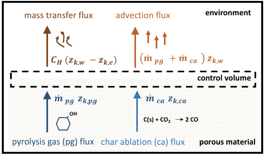
Surface mass balance at the heatshield front surface.
Under the assumption that Prandtl and Lewis numbers are equal to unity and the diffusion coefficients are identical between elements, the conservation of mass fraction of an element \(k\) in the control volume may be written as
The formation of the species \(S_i\) from the elements \(A_k\) is formulated as follows
Table 1.1 shows an example of the formation of the species from the and elements.
\(S_1\)
\(\nu_{1,1}\)
\(\nu_{1,2}\)
\(E_1\)
\(E_2\)
1
2
If the species are assumed perfect gas, then the chemical equilibrium is given by
The surface mass balance model computes \(\dot{m}_{ca}\) and \(h_w\) from Eq. [eq:massSurf1], [eq:massSurf2] and [eq:massSurf3].
The pyrolysis gas production rate at the heatshield front surface \(\dot{m}_{pg}\) by integrating the pyrolysis, mass and transport equations. \(p_w\) and \(C_H\) are given by the aerothermal environment. \(T_w\) and \(C'_H\) are computed in the surface energy balance described below.
The material mass loss rate leads to a surface ablation velocity given by
\[\vect{v}_{ca} = \frac{\dot{m}_{ca} }{\rho_{sw} } ~ \vect{n}\]and is applied as a mesh motion in PATO.
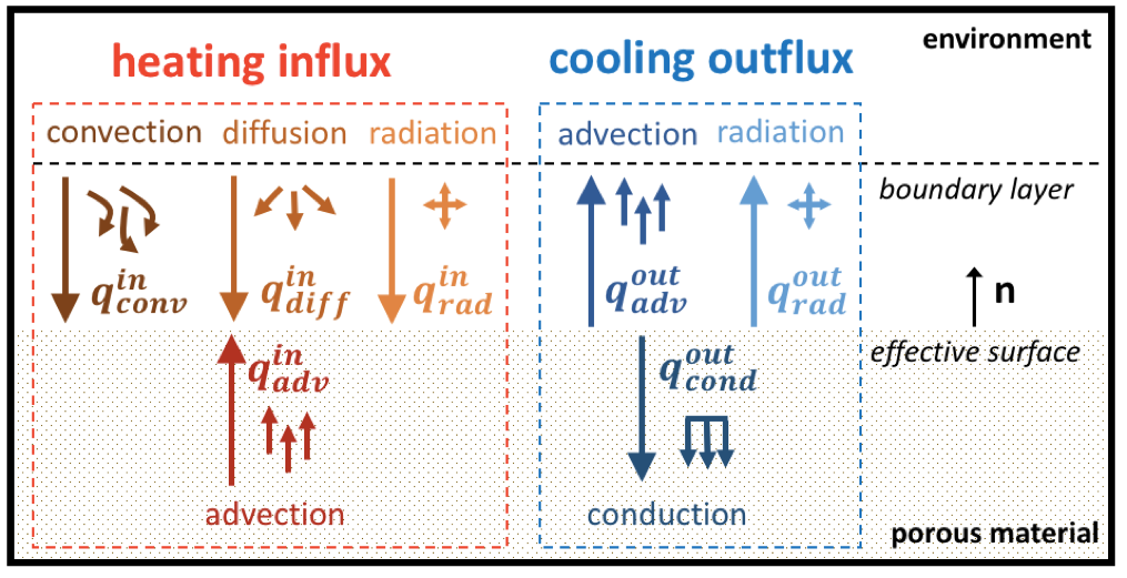
Surface energy balance at the heatshield front surface.
The equality between inward and outward fluxes yields
The different terms of Eq. [eq:in&out] are formulated here. The convective heat flux, under the assumption of a frozen boundary layer and a non-catalytic wall is
\(h_{ew}\) is the enthalpy computed at the wall temperature, with the boundary layer edge gaseous species composition.
The energy carried by diffusion of the gaseous species is given by
\(h_{w}\) is the enthalpy at the wall temperature, with the porous material gaseous species composition.
The advective energy transport produced by the pyrolysis and the char ablation read respectively
The radiative heating from the plasma is given by,
while the re-radiative cooling by surface emission reads
under the assumption that the surface behaves as a gray body.
The effective heat conduction in the porous material is given by
Eq. [eq:in&out], using the different energy contributions explained above, gives
Assuming equal Prandtl and Lewis number and equal diffusion coefficients for all elements, Eq. [eq:surfEnergy1] becomes
\(C_H\) is corrected to account only for the blockage induced by the pyrolysis and ablation gas blowing. The blowing correction (Eq. [eq:C’H]) is updated in the BlowingCorrection class where other film coefficient corrections, such as roughness and hot wall effects, are not considered.
\[\begin{aligned} \begin{split} &- \left(~ \overline{\overline{\vect{k}}}_w \cdot \frac{\partial T_w}{ \partial \vect{n}} \right) \cdot \vect{n} = h_{conv} \left( T_e - T_w \right) - \varepsilon_w \sigma \left( T_w^4 - T_{\infty}^4 \right) + \alpha_w q_{pla} \end{split} \label{eq:surfEnergyChemistryOff} \end{aligned}\]
optionsBC
The following optionsBC types are activated with a Switch in the BC input file:
factorOptionModel multiplies the fields from the first tuple elements in factorList by a factor equals to the second tuple elements.
timeFactorOptionModel updates the fields from the first tuple elements in timeFactorList using a linear interpolation of the data from timeFactorFile. The second tuple elements give the column indexes of the corresponding fields in timeFactorFile.
Listing [lis:optionBC] shows an example of the optionBC types. In this case, factorOptionModel multiplies by 2 the pressure boundary field of the top BC. timeFactorOptionModel updates the char blowing rate at the top BC using a linear interpolation in time of the first column values from constant/timeFactor.
boundaryField {
    top {
        type Bprime;
        factorOption yes;
        factorList (("p" 2));
        timeFactorOption yes;
        timeFactorFile "constant/timeFactor";
        timeFactorList (("BprimeCw" 1));
        BprimeFile "data/Materials/TACOT/BprimeTable";
        mappingType "constant";
        mappingFields ((p "1") (rhoeUeCH "2") (h_r "3"));
        Tbackground 187;
        qRad 0;
        lambda 0.5;
        chemistryOn 1;
        value uniform 300;
    }
}
BprimeCoating BC
The BprimeCoating BC extends the Bprime boundary condition for coated surfaces. While the underlying physics are identical with the ones of the previous section, the surface mass and energy balances are initially closed with the thermochemical parameters of the single component coating. Ablation of the material reduces the thickness of the coating till its complete removal, without deforming the mesh, an assumption justified by the fact that coatings are usually less than a millimeter in thickness. After the coating’s removal the substrate material is exposed and the boundary condition behaves like in the uncoated case.
BprimeCoatingMixture BC
The BprimeCoatingMixture BC is an extension of the BprimeCoating BC including multiple species coatings, such as Si-O-C (silicon oxycarbide) surfaces. The coating’s elemental composition needs to be specified, with the B’ tables calculated at run-time.
HeatFlux BC
The HeatFluxBoundaryConditions class applies a heat flux (\(q^{CFD}_{conv}\)) directly to the boundary. This boundary condition does not currently allow for recession. The surface energy balance is given by
erosionModel BC
The erosionModelBoundaryConditions class updates the cellMotionU field, which directly impacts the mesh motion. The physicsBasedErosionModel flag, chosen by the user, selects the type of erosion model.
type=1: the ablation rate is based on the minimum fiber radius failure and the gradient of fiber radius.
\[\boldsymbol{v}_{mesh} = \frac{r_{f,fail} - r_{f,w}}{\boldsymbol{\partial_x} r_{f,int} \cdot \boldsymbol{n} ~ \Delta t} ~ \boldsymbol{n}\]type=2: the ablation rate is based on the solid density gradient.
\[\boldsymbol{v}_{mesh} = \frac{50 - \rho_{s,w}}{\boldsymbol{\partial_x} \rho_{s,int} \cdot \boldsymbol{n}~ \Delta t} ~ \boldsymbol{n}\]type=3: the ablation rate is based on the cell-by-cell removing.
\[\boldsymbol{v}_{mesh} = 0.98 ~ \boldsymbol{v}_{mesh} + 0.02 ~ \frac{ \Delta x }{\Delta t} ~ \boldsymbol{n}\]type=4: the ablation rate is based on the solid density.
\[\boldsymbol{v}_{mesh} = \text{max}\left(1.05 ~ \boldsymbol{v}_{mesh} \cdot \boldsymbol{n} , ~\frac{10^{-7}}{\rho_{s,w}} \right) ~ \boldsymbol{n}\]type=5: the ablation rate is based on the heterogeneous rate.
\[\boldsymbol{v}_{mesh} = 0.95 ~ \boldsymbol{v}_{mesh} + 0.05 ~ \frac{\Omega_{H,int}}{\rho_{s,int}} ~ \boldsymbol{n}\]
coupledMixed BC
The coupledMixedFvPatchScalarField class creates the boundary conditions patch and updates the field \(f_1\) boundary conditions using the harmonic averaging of the neighbor field \(f_2\) (Eq. [eq:harmo]).
positiveGradient BC
The positiveGradientFvPatchScalarField class creates the boundary conditions patch and updates the field \(f_w\) boundary conditions using the cell center value \(f_1\) and the positive gradient (Eq. [eq:posGrad]).
pyro_recession BC
pyro_recession BC updates the mesh motion velocity \(\boldsymbol{v}_{mesh}\) using the recession rate \(r_r\).
radiative BC
The radiativeBoundaryConditions class updates the temperature BC. The wall temperature \(T_w\) is computed with a surface energy balance model (Eq. [eq:eb1]).
The convective heat flux, under the assumption of a frozen boundary layer and a non-catalytic wall is
\(h_{ew}\) is the enthalpy computed at the wall temperature, with the boundary layer edge gaseous species composition.
The energy carried by diffusion of the gaseous species is given by
\(h_{w}\) is the enthalpy at the wall temperature, with the porous material gaseous species composition.
The radiative heating from the plasma is given by,
while the re-radiative cooling by surface emission reads
under the assumption that the surface behaves as a gray body. The effective heat conduction in the porous material is given by
Eq. [eq:eb1], using the different energy contributions explained above, gives
Assuming equal Prandtl and Lewis number and equal diffusion coefficients for all elements, Eq. [eq:surfEnergy3] becomes
\(C_H\) is normally corrected to account for the blockage induced by the pyrolysis and ablation gas blowing. This radiativeBoundaryConditions class assumes there is no pyrolysis and ablation gas blowing.
The surface energy balance computes \(T_w\) from Eq. [eq:surfEnergy4] using the following user inputs: \(C_H\), \(h_e\), \(h_w\), \(\varepsilon_w\), \(T_\infty\), \(\alpha_w\) and \(q_{pla}\).
speciesBC BC
The speciesBCBoundaryConditions class updates the \(C'_H\) boundary conditions and reads the boundary layer edge species composition.
VolumeAblation BC
The VolumeAblationBoundaryConditions class updates the temperature boundary conditions and the mesh motion. The wall temperature \(T_w\) is computed with a surface energy balance model (Eq. [eq:eb1]).
The convective heat flux, under the assumption of a frozen boundary layer and a non-catalytic wall is
\(h_{ew}\) is the enthalpy computed at the wall temperature, with the boundary layer edge gaseous species composition.
The radiative heating from the plasma is given by,
while the re-radiative cooling by surface emission reads
under the assumption that the surface behaves as a gray body. The effective heat conduction in the porous material is given by
Eq. [eq:eb2], using the different energy contributions explained above, gives
type 1: the ablation rate is based on the minimum fiber radius failure and the gradient of fiber radius.
\[\boldsymbol{v}_{mesh} = \frac{r_{f,fail} - r_{f,w}}{\boldsymbol{\partial_x} r_{f,int} \cdot \boldsymbol{n} ~ \Delta t} ~ \boldsymbol{n}\]type 2: the ablation rate is based on the solid density gradient.
\[\boldsymbol{v}_{mesh} = \frac{50 - \rho_{s,w}}{\boldsymbol{\partial_x} \rho_{s,int} \cdot \boldsymbol{n}~ \Delta t} ~ \boldsymbol{n}\]type 3: the ablation rate is based on the cell-by-cell removing.
\[\boldsymbol{v}_{mesh} = 0.98 ~ \boldsymbol{v}_{mesh} + 0.02 ~ \frac{ \Delta x }{\Delta t} ~ \boldsymbol{n}\]type 4: the ablation rate is based on the solid density.
\[\boldsymbol{v}_{mesh} = \text{max}\left(1.05 ~ \boldsymbol{v}_{mesh} \cdot \boldsymbol{n} , ~\frac{10^{-7}}{\rho_{s,w}} \right) ~ \boldsymbol{n}\]type 5: the ablation rate is based on the heterogeneous rate.
\[\boldsymbol{v}_{mesh} = 0.95 ~ \boldsymbol{v}_{mesh} + 0.05 ~ \frac{\Omega_{H,int}}{\rho_{s,int}} ~ \boldsymbol{n}\]
basicWallHeatFluxTemperature BC
The basicWallHeatFluxTemperature BC applies a heat flux condition to temperature on a wall. It is based on the OpenFOAM externalWallHeatFlux BC. It operates in one of three modes:
Fixed power: supply Power \(Q\) in W.
\[\begin{split}\begin{align} T_{w} &= T_{cell}\\ \partial_w T &= \frac{\frac{Q}{S_f} + q_r}{k_s} \end{align}\end{split}\]Heat flux: supply heat flux \(q\) in W \(\cdot\) m\(^{-2}\).
\[\begin{split}\begin{align} T_{w} &= T_{cell}\\ \partial_w T &= \frac{q + q_r}{k_s} \end{align}\end{split}\]Fixed heat transfer coefficient: supply heat transfer coefficient \(h_{th}\) in W \(\cdot\) m\(^{-2} \cdot\) K\(^{-1}\) and ambient temperature \(T_{\infty}\) in K.
\[\begin{split}\begin{align} T_{w} &= \frac{h - \frac{q_r}{T_{cell}}}{h - \frac{q_r}{T_{cell}} + k_s ~ \frac{1}{\delta}} ~ \frac{\epsilon ~ \sigma ~ T^4}{h - \frac{q_r}{T_{cell}}} + \left( 1 - \frac{h - \frac{q_r}{T_{cell}}}{h - \frac{q_r}{T_{cell}} + k_s ~ \frac{1}{\delta}} \right) ~ T_{cell} \; &\text{if} \; q_r < 0\\ T_{w} &= \frac{h}{h + k_s ~ \frac{1}{\delta}} ~ \frac{\epsilon ~ \sigma ~ T^4 + q_r}{h} + \left( 1 - \frac{h}{h + k_s ~ \frac{1}{\delta}} \right) ~ T_{cell} \; &\text{if} \; q_r \geq 0 \end{align}\end{split}\]
darcyVelocityPressure BC
The darcyVelocityPressure BC provides a Darcy’s velocity condition for pressure. It is derived from a fixedGradient condition, whereas pressure is calculated from the projection of the velocity vector and permeability tensor on the direction of the flow.
darcyFlowRatePressure BC
The darcyFlowRatePressure BC provides a Darcy flow calculated for a uniform velocity field normal to the patch (Eq. [eq:darcyBC]) adjusted to match the specified flow rate. For a mass-based flux, the flow rate should be provided in kg \(\cdot\) s\(^{-1}\). For a volumetric-based flux, the flow rate is in m\(^3 \cdot s^{-1}\).
forchheimerVelocityPressure BC
The forchheimerVelocityPressure BC provides a compressible Darcy-Forchheimer’s velocity condition for pressure. It is derived from a fixedGradient condition, whereas pressure is calculated from the projection of the velocity vector and permeability tensor on the direction of the flow.
forchheimerFlowRatePressure BC
The forchheimerFlowRatePressure BC provides a compressible Darcy-Forchheimer’s flow calculated for a uniform velocity field normal to the patch (Eq. [eq:forchheimerBC]) adjusted to match the specified flow rate. For a mass-based flux, the flow rate should be provided in kg \(\cdot\) s\(^{-1}\). For a volumetric-based flux, the flow rate is in m\(^3 \cdot s^{-1}\).
tractionDisplacement BC
The tractionDisplacement BC provides a fixed traction BC for the standard linear elastic, fixed coefficient displacement equation with thermal and pyrolysis contribution.
fixedDisplacementZeroShear BC
The “fixedDisplacementZeroShear” BC sets the patch-normal component of displacement while allowing the two tangential directions to be free canceling any shear stress. The BC solves equation Eq. [eq:tracDis] and project its normal to the patch, setting the other components to zero.
qRad_emission_absorption BC
The qRad_emission_absorption BC updates the temperature boundary field at a patch using the radiative equilibrium condition. Other fields are mapped through BC.